Graphs and linearisation for practical data
Key idea: Choose graph axes from the physical model to make a straight line. Interpret its gradient and intercept with their units, and use lines consistent with the measurement allowances.
Offline pages
Saved on this device only. Connect at least once every 30 days to confirm Premium. Sign-out or a change of account removes saved copies.
Loading guide controls…
Guided lessons · coming soon
Guided lesson
Guided steps
- Choose axes that give the coefficients physical meaning.
- Read a large triangle on the fitted line.
- Follow the inverse-gradient calculation of g.
- Convert the gradient before finding the spring constant.
- Explain why length and extension have different intercepts.
- Find the cell constants and check the gradient sign.
- Predict whether any acceptable line must be limiting.
- Adjust the line and compare the allowed gradients.
- Explain how you tested both line conditions.
- Find the symmetric gradient allowance and g.
- Choose transformations from the proposed physical relationship.
- Choose the graph and find the force-model constants.
On this page
You stopped at:
ContinueA curved graph is hard to judge by eye, but a straight line can be tested and its gradient and intercept read off. Linearising means choosing what to plot so that the physical model becomes a straight line, then turning the gradient and intercept back into physical quantities with the right units.
Choose axes from the physical model
Start with the quantities you measured and the relationship you want to test, then decide what to plot so that the fitted coefficients have a physical meaning.
For a simple pendulum at small amplitude,
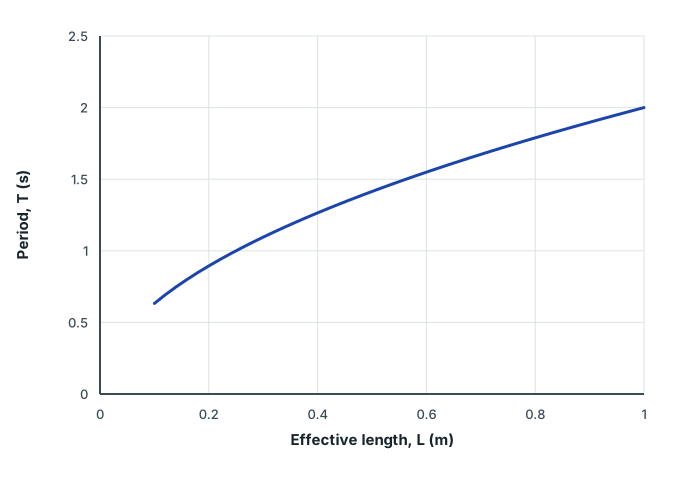
T is the period, L the effective pivot-to-centre-of-mass length and g the gravitational field strength. Assume g is constant and the pendulum is well approximated by a point mass on a light, inextensible suspension. A plot of T against L is curved. Squaring T gives a straight-line form whose gradient has a physical meaning.
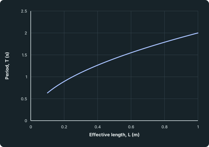
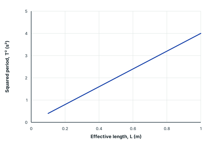
These two plots show the same ideal illustrative model, T² = 4.00L when T is in seconds and L in metres. They are calculated, not measured. This coefficient corresponds to g ≈ 9.87 m s⁻²; the interactive lab below uses a separate illustrative data set.
Period against length: an ideal curved model
For the illustrative model T² = 4.00L (seconds and metres), T increases with L but its gradient decreases. These are calculated model values, not measured observations.
Scroll across the figure to read all labels.
View figure data
| Effective length, L (m) | Period, T (s) |
|---|---|
| 0.10 | 0.6325 |
| 0.12 | 0.6928 |
| 0.14 | 0.7483 |
| 0.16 | 0.8000 |
| 0.18 | 0.8485 |
| 0.20 | 0.8944 |
| 0.22 | 0.9381 |
| 0.24 | 0.9798 |
| 0.26 | 1.0198 |
| 0.28 | 1.0583 |
| 0.30 | 1.0954 |
| 0.32 | 1.1314 |
| 0.34 | 1.1662 |
| 0.36 | 1.2000 |
| 0.38 | 1.2329 |
| 0.40 | 1.2649 |
| 0.42 | 1.2961 |
| 0.44 | 1.3266 |
| 0.46 | 1.3565 |
| 0.48 | 1.3856 |
| 0.50 | 1.4142 |
| 0.52 | 1.4422 |
| 0.54 | 1.4697 |
| 0.56 | 1.4967 |
| 0.58 | 1.5232 |
| 0.60 | 1.5492 |
| 0.62 | 1.5748 |
| 0.64 | 1.6000 |
| 0.66 | 1.6248 |
| 0.68 | 1.6492 |
| 0.70 | 1.6733 |
| 0.72 | 1.6971 |
| 0.74 | 1.7205 |
| 0.76 | 1.7436 |
| 0.78 | 1.7664 |
| 0.80 | 1.7889 |
| 0.82 | 1.8111 |
| 0.84 | 1.8330 |
| 0.86 | 1.8547 |
| 0.88 | 1.8762 |
| 0.90 | 1.8974 |
| 0.92 | 1.9183 |
| 0.94 | 1.9391 |
| 0.96 | 1.9596 |
| 0.98 | 1.9799 |
| 1.00 | 2.0000 |
Squared period against length: the same model
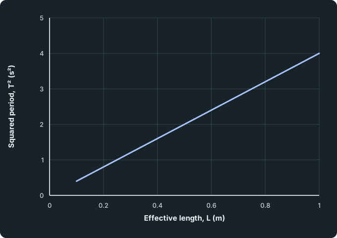
Squaring the period gives a straight-line trend with zero model intercept for the same ideal model. Its gradient is 4.00 s² m⁻¹, corresponding to g ≈ 9.87 m s⁻²; this does not prove that measured data have zero intercept.
Scroll across the figure to read all labels.
View figure data
| Effective length, L (m) | Squared period, T² (s²) |
|---|---|
| 0.10 | 0.40 |
| 0.12 | 0.48 |
| 0.14 | 0.56 |
| 0.16 | 0.64 |
| 0.18 | 0.72 |
| 0.20 | 0.80 |
| 0.22 | 0.88 |
| 0.24 | 0.96 |
| 0.26 | 1.04 |
| 0.28 | 1.12 |
| 0.30 | 1.20 |
| 0.32 | 1.28 |
| 0.34 | 1.36 |
| 0.36 | 1.44 |
| 0.38 | 1.52 |
| 0.40 | 1.60 |
| 0.42 | 1.68 |
| 0.44 | 1.76 |
| 0.46 | 1.84 |
| 0.48 | 1.92 |
| 0.50 | 2.00 |
| 0.52 | 2.08 |
| 0.54 | 2.16 |
| 0.56 | 2.24 |
| 0.58 | 2.32 |
| 0.60 | 2.40 |
| 0.62 | 2.48 |
| 0.64 | 2.56 |
| 0.66 | 2.64 |
| 0.68 | 2.72 |
| 0.70 | 2.80 |
| 0.72 | 2.88 |
| 0.74 | 2.96 |
| 0.76 | 3.04 |
| 0.78 | 3.12 |
| 0.80 | 3.20 |
| 0.82 | 3.28 |
| 0.84 | 3.36 |
| 0.86 | 3.44 |
| 0.88 | 3.52 |
| 0.90 | 3.60 |
| 0.92 | 3.68 |
| 0.94 | 3.76 |
| 0.96 | 3.84 |
| 0.98 | 3.92 |
| 1.00 | 4.00 |
Squaring changes the vertical quantity and its unit. It does not create more accurate measurements. For small fractional period uncertainty, Δ(T²) ≈ 2TΔ T; carry the transformed allowance into the new graph. For a larger allowance, transform the endpoints (T-Δ T)² and (T + Δ T)² while keeping the physically positive period range.
Choosing a fit and reading its gradient
Label each axis with the plotted quantity and unit. Choose simple scales that use much of the available graph paper. Include zero when it helps you interpret an intercept; you do not have to sacrifice the data range to include it on every graph.
Fit the overall trend rather than joining successive points. Inspect residuals—the differences between observations and fitted values—for a pattern or an unusual point. Investigate an apparent anomaly before excluding it. Curved residuals can indicate that a straight-line model does not describe the tested range.
Use two well-separated coordinates on the fitted line for a manual gradient:
A large triangle reduces the relative effect of coordinate-reading uncertainty. Its corners do not need to be measured points. The gradient unit is the vertical-axis unit divided by the horizontal-axis unit; the intercept has the vertical-axis unit. Compare the physical equation with Y = mX + c before interpreting either coefficient.
Do not force a line through the origin just because the ideal equation has no intercept. First consider offsets, uncertainty and whether the model describes the apparatus. A justified zero-intercept fit and a free-intercept fit answer different questions.
Worked example 1
Turn a pendulum gradient into g
Problem
Show full solution
Calculate the gradient
Method
m = 4.00 s² m⁻¹.Reason
The triangle uses changes on the fitted line and the axis units determine the gradient unit.Working
Answer
m = 2.40/0.600 = 4.00 s² m⁻¹Match the coefficient
Method
m = 4π²/g, so g = 4π²/m.Reason
Compare T² = mL + c with the small-angle model; the gradient is inversely proportional to g.Working
Answer
g = 4π²/(4.00 s² m⁻¹) = 9.87 m s⁻²
Quick check
Guided practice 2
Spring length against force
Problem
Try this before viewing the solution
Show the steps Optional working
Hints
Hint 1
Match the length unit
Convert centimetres to metres before taking the inverse gradient.Hint 2
Compare coefficients
Write L = L₀ + (1/k)F and compare it with Y = c + mX.Show solution step by step
Convert before taking the inverse
Method
The SI gradient is 0.0400 m N⁻¹.Reason
The plotted length is in centimetres, while k is required in newtons per metre.Working
Answer
4.00 cm N⁻¹ = 0.0400 m N⁻¹Read the coefficient and constant term
Method
k = 25.0 N m⁻¹ and L₀ = 5.00 cm.Reason
For length against force the gradient is 1/k in SI units; the zero-force intercept is the unloaded length.Working
Answer
k = 1/0.0400 = 25.0 N m⁻¹
Quick check
Check your understanding 1 What does the spring intercept mean?
For the graph above, explain the 5.00 cm intercept. Would a graph of extension against force have the same intercept? State when the straight-line model applies.
Show answer
The length intercept is the unloaded length L₀ = 5.00 cm. Extension is x = L-L₀, so its ideal force graph has zero extension at zero force. Both have the same SI gradient 1/k when length or extension is vertical and force horizontal. The line applies within the spring’s Hooke’s-law range. Compare your answer for the quantity on the vertical axis, the zero-force value and the range of proportional extension.
Check your understanding 2 Transfer to a discharging cell
For constant e.m.f. E and internal resistance r, V = E-rI. An illustrative graph of terminal p.d. V/V against current I/A has gradient -0.80 V A⁻¹ and intercept 1.50 V. Find E and r. Would a positive gradient agree with this model for positive discharge current?
Show answer
E = 1.50 V and r = -m = 0.80 Ω, since V A⁻¹ = Ω. A positive gradient would imply negative r in this model; check polarity, current direction, measurements and model conditions rather than accepting that as an ordinary positive resistance. Changes in temperature or cell condition can make constant E and r unsuitable.
Compare lines within vertical allowances
Check your understanding 3 Predict before moving the line
If a straight line crosses every vertical allowance, must it be a limiting line with the largest or smallest possible gradient?
Show answer
No. Many gradients may cross all the allowances with a suitable intercept. A limiting line reaches the steepest or shallowest gradient that still crosses every allowance; an arbitrary crossing line can lie inside that range.
Try an acceptable line and a limiting line
The lab supplies its own illustrative observations. Adjust the solid line to the overall trend. Select Include zero on both axes to see the intercept, then compare the dotted unweighted least-squares reference. That reference minimises squared vertical residuals; it does not weight observations by their different allowances.
Turn on Explore a limiting line. Adjust the dashed trial until it crosses every vertical allowance and approaches either end of the displayed allowed-gradient range. Drag the ends, or focus a handle and use the arrow keys; Shift moves faster. Explain why a line can cross every allowance yet still lie inside the limiting gradients.
Pendulum: T² against l. Small-angle pendulum: T² = (4π²/g)l; l is pivot-to-centre-of-mass length. A positive gradient is required. Fixed x values; separate vertical allowances; free intercept. These bounds do not include x uncertainty or shared calibration errors and are not statistical confidence limits. Your solid line: gradient 2.82 s^2 m^{−1}, intercept 0.998 s^2. Actual illustrative observations (x, y ± allowance): 0.200 m, 0.8197 s^2 ± 0.0541 s^2; 0.350 m, 1.390 s^2 ± 0.0723 s^2; 0.500 m, 2.001 s^2 ± 0.0904 s^2; 0.650 m, 2.655 s^2 ± 0.108 s^2; 0.800 m, 3.227 s^2 ± 0.127 s^2; 0.950 m, 3.823 s^2 ± 0.145 s^2.
- Gradient of your line
- 2.82 s2 m−1
- y-intercept of your line
- 0.998 s2
- Gradient of the limiting-line trial
- 4.44 s2 m−1
- Gradient allowance covering both limits
- —
- Allowed gradient range
- 3.740 s2 m−1 to 4.270 s2 m−1
- Limiting-line trial
- Misses at least one vertical allowance
- Model, units and fit condition
- Small-angle pendulum: T² = (4π²/g)l; l is pivot-to-centre-of-mass length. A positive gradient is required. The solid line misses at least one vertical allowance; its gradient allowance is unavailable.
- Illustrative data: x, y ± vertical allowance
- 0.200 m: 0.8197 s2 ± 0.0541 s2; 0.350 m: 1.390 s2 ± 0.0723 s2; 0.500 m: 2.001 s2 ± 0.0904 s2; 0.650 m: 2.655 s2 ± 0.108 s2; 0.800 m: 3.227 s2 ± 0.127 s2; 0.950 m: 3.823 s2 ± 0.145 s2
- From your line
- g = 14.0 m s⁻²
Try this
0 of 4 doneDrag the ends of the line until it is a good best fit. (not done yet)
Judge the overall trend and residuals. Here a compatible best-fit line also crosses every vertical allowance; it need not pass through any point or the origin. The dotted reference is unweighted least squares, not an uncertainty-weighted fit.
Bring the trial line close to either limiting gradient while crossing every vertical allowance. (not done yet)
For fixed x values and a free intercept, the allowed range is calculated using every vertical allowance. The task accepts a line within 5% of that slope span from either limit. A symmetric allowance around a compatible best fit must cover the farther limit; these are not confidence limits.
Use the pendulum data to find g within 2% of 9.81 m s⁻². (not done yet)
T² = (4π² / g) l, so g = 4π² / gradient. A large gradient triangle reduces the error in reading it.
Use the cell data to find the e.m.f. from the y-intercept, within 0.03 V. (not done yet)
V = E − I r: the intercept on the V-axis (I = 0) is the e.m.f. and the gradient is −r.
You’ve tried every task.
Check your understanding 4 Explain what your line shows
Record your best-fit gradient and the allowed-gradient range from the lab. Explain how you decided whether your dashed line was acceptable and whether it was limiting. If the lab is unavailable, sketch a set of vertical allowances and describe the two tests.
Show answer
An acceptable line crosses every vertical allowance. A limiting line does that and reaches either end of the feasible gradient range. Moving one end changes both gradient and intercept, so check every allowance again. Compare your explanation for both tests and the range shown by your own lab trial; the lab’s data differ from the ideal worked example. These limits use exact horizontal coordinates and separate vertical allowances, rather than a statistical confidence interval.
This simplified construction treats x as exact, allows a free intercept and treats each vertical allowance separately. The lab calculates the full feasible slope range using all observations. If you report a symmetric allowance around a compatible best-fit gradient, use the larger distance to the minimum or maximum slope. Trying just one arbitrary acceptable line can understate that allowance.
These limits are not statistical confidence intervals and do not account for horizontal uncertainty or shared calibration errors. Follow the method stated in your practical task, and explain the assumptions behind your own estimate. This activity develops graph judgement; it does not replace collecting real data or using a spreadsheet.
Check your understanding 5 Choose a symmetric gradient allowance
For a T² against L graph, a compatible best-fit gradient is 4.10 s² m⁻¹. The feasible gradients run from 3.84 to 4.23 s² m⁻¹. Find the smallest symmetric allowance about 4.10 that covers the full range, and calculate g from the best-fit gradient.
Show answer
The distances are 4.10-3.84 = 0.26 and 4.23-4.10 = 0.13 s² m⁻¹. Use ±0.26 s² m⁻¹ around 4.10 to cover both ends. Half the feasible range, 0.195, would be centred at 4.035 instead and would not cover the lower end when centred at 4.10. The best-fit estimate is g = 4π²/4.10 = 9.63 m s⁻².
Other ways to linearise a model
Choose a transformation from a proposed model and define the transformed quantities before plotting. A logarithm acts on a positive dimensionless ratio. Here x_ref and y_ref are fixed positive reference quantities with the same units as x and y.
| Model | Linear plot: vertical against horizontal | Gradient |
|---|---|---|
| y = kxⁿ, with known n | y against xⁿ | k, with unit [y]/[x]ⁿ |
| y = y₀e^kx, with y,y₀ > 0 | ln(y/y₀) against x | k, with unit [x]⁻¹ |
| y = axⁿ, with unknown n and positive x,y | ln(y/y_ref) against ln(x/x_ref) | n, dimensionless |
| y = a/x + b, with x ≠ 0 | y against 1/x | a, with unit [y][x] |
For the power law, the intercept is ln(a x_refⁿ/y_ref). Changing reference quantities changes the intercept but not n. With natural logarithms the exponential gradient is k; using base-10 logarithms instead gives k/ln 10. State the base consistently. A logarithmic power-law gradient still gives n when both axes use the same base.
For small uncertainty, Δ ln(y/y_ref) ≈ Δ y/y, so a constant absolute y allowance generally does not stay constant after a log transformation. If an interval includes zero, its logarithm is not a valid finite transformed interval. Similarly, inversion and powers can produce asymmetric transformed intervals; check endpoint values and the allowed domain.
Check your understanding 6 A new force model
An investigation tests F = a xⁿ, with positive extension x. It gives F = 0.160 N at x = 0.0200 m and F = 0.640 N at x = 0.0400 m. Choose a straight-line plot for finding the unknown exponent. Use F_ref = 1 N and x_ref = 1 m for any logs. Find n, then the numerical value of a in SI units and its unit.
Show the steps Optional working
Show answer
Take Y = ln(F/F_ref) and X = ln(x/x_ref). Then Y = nX + ln(a x_refⁿ/F_ref). The gradient is n = ln(0.640/0.160)/ln(0.0400/0.0200) = ln 4/ln 2 = 2. Thus a = F/x² = 0.160/(0.0200)² = 400 N m⁻², matching the second record. These two points are consistent with the model; more data across a suitable range are needed to test its shape.
Common mistakes
- Reporting the gradient as the physical quantity. For T² against L the gradient is 4π²/g, so g = 4π²/m.
- Using data points that are not on the line for the gradient triangle. Read two well-separated points on the fitted line.
- Forgetting a unit conversion before inverting a gradient. A gradient in cm N⁻¹ must be converted to m N⁻¹ before finding k.
- Forcing the line through the origin because the ideal equation has no intercept. Check offsets and uncertainty first.
- Keeping the same error bar after transforming a quantity. Squaring, inverting or taking logarithms changes the allowance.
- Taking the logarithm of a quantity with units. Take the log of a dimensionless ratio, such as y/y_ref.
Spotted an error? Report a correction
Syllabus and review details
- GCE A-Level H2 Physics 2027 · 2027
Content Overview, PDF pages 9–10; Subject Content, PDF pages 11–30