Charge Transport and Resistivity
Key idea: Advanced Physics: current density and drift velocity, the Drude relaxation-time model of conductivity, resistance versus resistivity, how metal resistivity depends on temperature, and choosing conductor materials.
Continue where you stopped
The core idea
On this page
Learning objectives
- Connect energy bands, carrier response, Hall measurements, and semiconductor-device behaviour.
This lesson connects the band picture from the previous lesson to measurable currents. It builds a microscopic model of conduction, tests it against how real metals behave, and sets up the carrier density and drift velocity that the Hall effect measures next.
Use this page for:
- relating current to carrier density and drift velocity,
- the Drude relaxation-time model of conductivity and where it fails,
- separating material (resistivity) from shape (resistance),
- reading how a metal’s resistivity changes with temperature,
- choosing a conductor from its properties.
Prerequisites: H2 current electricity and Energy Band Structures In Solids.
Fast start
- Current in a conductor is I = n|q|Av_d, and current density is J = nqv_d.
- The drift velocity is tiny, typically below 1 mm s⁻¹ in a metal wire. The electrical signal travels roughly 10¹¹ times faster.
- The Drude model gives σ = nq²τ/m and ρ = 1/σ. It explains Ohm’s law but not the temperature dependence of metals.
- Resistivity belongs to the material and its temperature; resistance also depends on shape through R = ρ L/A.
- A metal’s resistivity is a nearly constant residual value at very low temperatures and rises roughly linearly near room temperature. Semiconductors behave differently.
1. Current from moving carriers
Take a conductor of cross-sectional area A containing n mobile charge carriers per unit volume, each with charge q. In an electric field the carriers acquire a small average velocity along the conductor, the drift velocity v_d, on top of their much faster random motion.
First consider magnitudes. In a time Δ t, drift transports a net number nAv_dΔ t of carriers across a chosen cross-section, where v_d is the drift speed. Random motion carries particles both ways and contributes no net current in this model. The magnitude of the transported charge is Δ Q = n|q|Av_dΔ t, giving
I = (Δ Q)/(Δ t) = n|q|Av_d.
The current density is the current per unit cross-sectional area:
J = nqv_d, J = I/A.
Sign convention used in this lesson. In vector equations, q is signed and v_d is a velocity: electrons have q = -e and drift opposite to the field. When you only need sizes, as in most calculations, use magnitudes: I = n|q|Av_d. The product qv_d points along the field whatever the sign of the carriers, so current direction alone cannot tell you the sign of the carriers. The Hall effect can.
| Quantity | Symbol | SI unit |
|---|---|---|
| Carrier number density | n | m⁻³ |
| Carrier charge | q | C |
| Drift speed | v_d | m s⁻¹ |
| Current density | J | A m⁻² |
Worked example: how fast do electrons drift? A copper wire of cross-sectional area 1.5 mm² carries 10 A. Copper has about one free electron per atom, so n = 8.5 × 10²⁸ m⁻³.
v_d = I/n|q|A = 10/((8.5 × 10²⁸)(1.6 × 10⁻¹⁹)(1.5 × 10⁻⁶)) = 4.9 × 10⁻⁴ m s⁻¹.
That is about half a millimetre per second, so an electron would take over half an hour to drift one metre. A lamp still lights almost as soon as the switch closes, because the change in the electric field propagates along the circuit at a speed of order 10⁸ m s⁻¹, depending on the cable and surrounding dielectric. Carriers already near the lamp respond when that change reaches them; electrons do not have to drift all the way from the switch. Keep three things apart: the carriers’ fast random motion, their slow drift, and the fast but finite spread of the field that we call the signal.
Try it first. An aluminium wire of cross-sectional area 2.0 mm² carries 5.0 A. Aluminium supplies about three free electrons per atom, so n = 1.8 × 10²⁹ m⁻³. Find the drift speed. Would a copper wire of the same area carrying the same current have a larger or smaller drift speed?
Check your drift speed
v_d = 5.0/[(1.8 × 10²⁹)(1.6 × 10⁻¹⁹)(2.0 × 10⁻⁶)] = 8.7 × 10⁻⁵ m s⁻¹. For the same I and A, the drift speed is inversely proportional to n. Copper has fewer free electrons per cubic metre, so its electrons must drift faster, about 1.8 × 10²⁹/8.5 × 10²⁸ ≈ 2.1 times faster.
2. The Drude model of conduction
In 1900 Paul Drude modelled the free electrons in a metal as a classical gas of particles moving through a lattice of positive ions. The model makes four assumptions:
- between collisions, each carrier moves freely and responds only to the applied field;
- a collision instantly randomises the carrier’s velocity, so on average it keeps no memory of its earlier drift;
- the mean time between collisions, the relaxation time τ, does not depend on the field or on the carrier’s velocity;
- the carriers obey classical mechanics.
From field to drift velocity. Between collisions, a carrier accelerates at a = qE/m. Just after a collision its velocity averages to zero over all carriers. At any instant, carriers have been accelerating for an average time τ since their last collision, so the average velocity they have gained is
v_d = qEτ/m.
Collisions act like a drag that stops the drift growing without limit, which is why a steady field gives a steady current.
From drift velocity to conductivity. Substitute into J = nqv_d:
J = nq²τ/m E = σE, σ = nq²τ/m, ρ = 1/σ = m/nq²τ.
Because τ does not depend on E, J is proportional to E. This is Ohm’s law. The factor q² also shows that J is along E for either sign of carrier.
Worked example: how often do electrons scatter in copper? At room temperature copper has ρ = 1.68 × 10⁻⁸ Ω m. Rearranging for τ:
τ = m/nq²ρ = (9.11 × 10⁻³¹)/((8.5 × 10²⁸)(1.6 × 10⁻¹⁹)²(1.68 × 10⁻⁸)) = 2.5 × 10⁻¹⁴ s.
Older treatments write the model in terms of a mean free path λ instead of τ. The two are linked by λ = v bar τ, where v bar is the carriers’ average random speed, not the drift speed. Substituting gives ρ = mv bar/(nq²λ), which is the same model written differently. Do not mix the two forms in one derivation without stating this link.
Where the classical model fails
The Drude model gets the size of the conductivity roughly right, but it fails several tests.
- Temperature dependence. Suppose, as Drude did, that λ is fixed by the ion spacing and that v bar is the classical thermal speed, which is proportional to square root of T. Then ρ ∝ square root of T. For most pure metals near room temperature, ρ is observed to rise roughly in proportion to T instead (section 4).
- Mean free path. With the classical thermal speed at 300 K, about 1.2 × 10⁵ m s⁻¹, the value of τ above gives λ ≈ 3 nm, already about ten ion spacings. Very pure copper near 4 K has a resistivity roughly a thousand times smaller, which implies free paths of micrometres. Electrons cannot be bouncing off every ion.
- Materials it cannot classify. Nothing in the model explains why diamond is an insulator or why a semiconductor conducts better when heated. The band picture from the previous lesson does.
- Carrier sign. Some metals and many semiconductors give Hall voltages of the “wrong” sign for free electrons, which you will meet in the next lesson.
The quantum picture fixes these problems without discarding σ = nq²τ/m. Electrons behave as waves. A wave passes through a perfectly regular lattice without scattering, so collisions come only from departures from perfect order. Only electrons near the Fermi level can change state, and they move at the Fermi speed of about 1.6 × 10⁶ m s⁻¹ in copper, not at a thermal speed. This lesson stops at that qualitative picture.
3. Resistance and resistivity
Resistivity ρ is a property of a material at a given temperature. Resistance R is a property of a particular object. For a uniform conductor of length L and cross-sectional area A,
R = (ρ L)/A.
This separates two different decisions:
- Changing the material or its temperature changes ρ, so it changes R for the same shape.
- Changing the shape (a longer wire or a thinner wire) changes R but leaves ρ unchanged.
Resistivity has units of Ω m, not Ω m⁻¹. A useful check is that ρ = RA/L has units Ω × m² / m.
Worked example. A 20 m length of copper cable has conductors of cross-sectional area 1.5 mm². Find the resistance of one conductor at room temperature.
R = (ρ L)/A = ((1.68 × 10⁻⁸)(20))/(1.5 × 10⁻⁶) = 0.22 Ω.
The current flows out along one conductor and back along the other, so the circuit loop contains 40 m of copper and has a resistance of about 0.45 Ω.
Try it first. A nichrome heating wire is 0.50 m long with a diameter of 0.40 mm. At its working temperature its resistivity is 1.10 × 10⁻⁶ Ω m.
- Find its resistance.
- Find the resistance of a 1.00 m length of the same wire.
- The wire is then run hotter, and its resistivity rises by 2%. Find the new resistance of the 0.50 m length.
Check your resistances
- A = π(0.20 × 10⁻³)² = 1.26 × 10⁻⁷ m², so R = (1.10 × 10⁻⁶)(0.50)/(1.26 × 10⁻⁷) = 4.4 Ω.
- Doubling the length is a geometric change. The resistivity is unchanged and R doubles to 8.8 Ω.
- A temperature change is a material change. The shape is unchanged, so R rises by the same 2%, to 4.5 Ω.
If you changed ρ in part 2, you treated a change of shape as a change of material.
4. How a metal’s resistivity depends on temperature
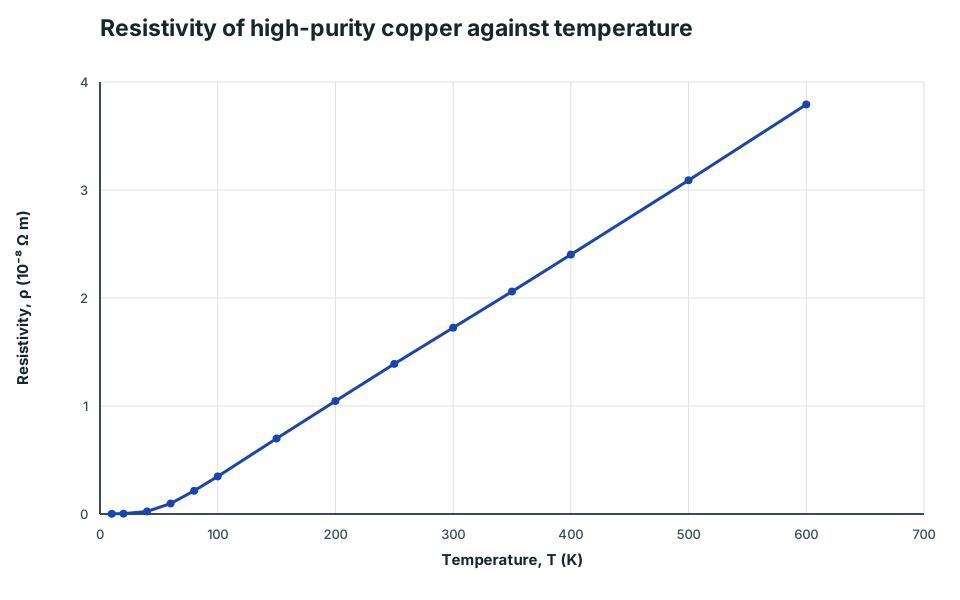
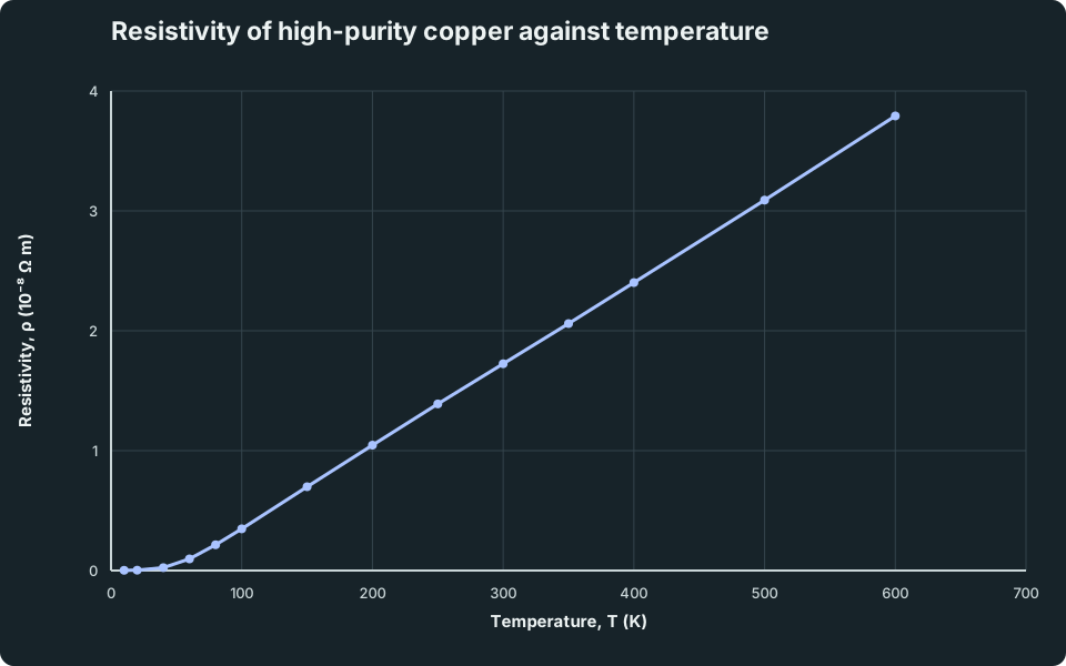
Resistivity of high-purity copper against temperature
Resistivity of high-purity copper from 10 K to 600 K. The resistivity is almost zero and nearly constant below about 20 K, rises increasingly steeply up to about 100 K, and then rises steadily to 3.79 × 10⁻⁸ Ω m at 600 K.
Scroll across the graph to read all labels.
View figure data
| Temperature, T (K) | High-purity copper (illustrative) |
|---|---|
| 10 | 0.002 |
| 20 | 0.003 |
| 40 | 0.024 |
| 60 | 0.097 |
| 80 | 0.215 |
| 100 | 0.348 |
| 150 | 0.699 |
| 200 | 1.046 |
| 250 | 1.39 |
| 300 | 1.725 |
| 350 | 2.06 |
| 400 | 2.402 |
| 500 | 3.09 |
| 600 | 3.792 |
In a metal the number of free electrons hardly changes with temperature, so any change in ρ comes from a change in scattering. Two kinds of disorder scatter the electron waves:
- Lattice vibrations. The ions vibrate more as the temperature rises. Well above a few tens of kelvin, this contribution ρ_lattice is roughly proportional to T. At very low temperatures it falls away rapidly.
- Static defects and impurities. Impurity atoms, vacancies and grain boundaries do not depend on temperature. They give a constant residual resistivity ρ_residual.
To a good approximation the two contributions add (Matthiessen’s rule):
ρ(T) = ρ_residual + ρ_lattice(T).
Over a limited range near room temperature, the rise is close to linear and is often written
ρ ≈ ρ₀[1 + α(T - T₀)],
where ρ₀ is the resistivity at a reference temperature T₀ and α is the temperature coefficient of resistivity. This is an empirical fit over a stated range, not a law.
- At low temperatures a metal’s resistivity levels off at its residual value.
- For a semiconductor the carrier density n rises steeply with temperature, so the resistivity usually falls as it is heated.
- Alloys such as nichrome have a large residual part, so their resistivity changes much less with temperature than a pure metal’s does.
Try it first. Use the graph or its data table.
- Calculate the gradient of the graph between 200 K and 400 K. Use it to estimate α for copper at 300 K.
- A student extends the straight line through the 200 K and 400 K points back to 0 K. What resistivity does that predict, and what does the result tell you about the linear model?
- Sketch how the curve would change for a copper sample containing more impurities.
Check your graph reasoning
- Gradient = (2.402 - 1.046)/(400 - 200) = 6.78 × 10⁻³ in units of 10⁻⁸ Ω m K⁻¹. Then α = (dρ/dT)/ρ = 6.78 × 10⁻³/1.725 = 3.9 × 10⁻³ K⁻¹, which is the usual value quoted for copper near room temperature.
- ρ(0) = 1.046 - 200 × 6.78 × 10⁻³ = -0.31, in units of 10⁻⁸ Ω m. A negative resistivity is impossible. The line reaches zero at about 46 K, while the data level off at a small positive residual value instead. The linear model only describes the range where lattice scattering is roughly proportional to T.
- More impurities raise the residual resistivity, so the whole curve moves up by roughly a constant amount. At high temperatures its slope is almost unchanged, because the lattice contribution is the same.
5. Choosing a conductor material
Resistivity is rarely the only property that matters. The table gives typical values near 20 °C; exact values depend on the grade and on heat treatment. The International Annealed Copper Standard (IACS) defines 100% conductivity as ρ = 1.724 × 10⁻⁸ Ω m.
| Material | Resistivity / 10⁻⁸ Ω m | Density / kg m⁻³ | Other relevant properties |
|---|---|---|---|
| Silver | 1.59 | 10 500 | Lowest resistivity of any metal; expensive; tarnishes |
| Copper (annealed) | 1.68 | 8 960 | Ductile and easy to join; soft when annealed |
| Aluminium (conductor grade) | 2.8 | 2 700 | About 61% IACS; low density; low tensile strength |
| Beryllium copper (high-strength grade) | about 7–8 | 8 250 | About 20–25% IACS; strong and springy |
| Nichrome (approximately 80% Ni, 20% Cr) | about 110 | 8 300 | Resists oxidation when red hot; small temperature coefficient |
These numbers replace two common slogans. Aluminium is not simply “half as good” as copper. For the same cross-section it conducts about 60% as well, but for the same resistance per metre it has about half the mass. Beryllium copper is not “close to copper” either: high-strength grades conduct only about a quarter as well, and they are used where springiness and strength matter more than conductivity.
For grade-specific comparisons, Nexans’ conductor-property table gives 1350-H19 aluminium at a minimum 61% IACS and half the mass of the IACS copper reference at equal length and DC resistance. The Copper Development Association’s C17200 data give a typical conductivity of 22% IACS for that high-strength copper–beryllium alloy. Kanthal’s Nikrothal 80 data sheet gives a density of 8.30 g cm⁻³ and resistivity of 1.09 Ω mm² m⁻¹ at 20 °C, and describes its oxidation resistance. The rounded values above support the comparisons here; an actual design needs the chosen grade’s data at its operating temperature.
Try it first. An overhead power line must have a resistance of no more than 0.10 Ω per kilometre of conductor.
- For copper and for aluminium, find the cross-sectional area needed and the mass of one kilometre of conductor.
- Which would you choose for a long overhead span, and what property in the table still needs addressing?
- A 230 V, 1.0 kW heater element uses wire of cross-sectional area 0.20 mm². For an initial material comparison, use the table’s room-temperature resistivities to estimate the lengths of nichrome and copper wire needed, and give a second reason why copper is unsuitable. A finished design must use resistivity at its operating temperature.
Check your material choices
- A = ρ L/R. For copper, A = (1.68 × 10⁻⁸)(1000)/0.10 = 1.7 × 10⁻⁴ m² (168 mm²), with mass 8960 × 1.68 × 10⁻⁴ × 1000 ≈ 1500 kg. For aluminium, A = 2.8 × 10⁻⁴ m² (280 mm²), with mass 2700 × 2.8 × 10⁻⁴ × 1000 ≈ 760 kg.
- Aluminium: it needs a thicker conductor but has about half the mass, so the towers can be lighter or further apart. Its low tensile strength remains a problem, which is why overhead lines usually wind aluminium strands around a steel core.
- The element needs R = V²/P = 230²/1000 = 53 Ω, so L = RA/ρ. Nichrome: L = (53)(0.20 × 10⁻⁶)/(1.10 × 10⁻⁶) ≈ 9.6 m. Copper: L = (53)(0.20 × 10⁻⁶)/(1.68 × 10⁻⁸) ≈ 630 m. Copper would also oxidise rapidly at red heat, while nichrome forms a protective oxide layer.
6. From transport to Hall measurements
In this lesson n was taken from the number of free electrons per atom. The next lesson measures it. A magnetic field deflects the drifting carriers sideways and sets up a Hall voltage V_H = BI/(n|q|t) across a sample of thickness t. Its polarity reveals the sign of q.
Try it first. A copper strip 0.10 mm thick carries 5.0 A at right angles to a 1.0 T magnetic field.
- Using n = 8.5 × 10²⁸ m⁻³, predict the size of the Hall voltage.
- A doped semiconductor strip of the same thickness has n = 1.0 × 10²² m⁻³ and carries 5.0 mA in the same field. Compare its Hall voltage and explain why Hall probes are made from semiconductors.
Check your prediction
- V_H = (1.0)(5.0)/[(8.5 × 10²⁸)(1.6 × 10⁻¹⁹)(1.0 × 10⁻⁴)] = 3.7 × 10⁻⁶ V, only about 4 µV. The carrier density is so large that the carriers drift slowly, so the sideways force on each one is small.
- V_H = (1.0)(5.0 × 10⁻³)/[(1.0 × 10²²)(1.6 × 10⁻¹⁹)(1.0 × 10⁻⁴)] = 31 mV, nearly ten thousand times larger even with a thousandth of the current. A much smaller n means a much larger drift speed for a given current, so the Hall voltage is easy to measure.
Next steps
Continue with the next resource in this course.
Course and syllabus information
- Course
- Advanced Physics
- Edition
- Advanced Physics