Background radiation and half-life

Syllabus and review details

• K326 / K327 Science Physics componentK326 / K327 · 2027Checked against the syllabus · partial topic coverageRadioactivity topic 16(a)–(h), PDF pages 23–24

Separate the source from its surroundings

A detector records radiation from the source and background radiation from the environment. Background sources include cosmic rays, rocks and building materials, and naturally occurring radioactive substances in living things.

Those are natural sources. Artificial sources, such as operating medical X-ray equipment, can also contribute to radiation detected in the surroundings.

To compare readings fairly, use the same detector position and settings. Convert counts to count-rate before subtracting readings taken over different durations:

count-rate = counts/(counting time).

For example, a background observation of 100 counts in 5 minutes gives 20 counts/min. A source-present observation of 260 counts in 1 minute gives 260 counts/min. The estimated source contribution is 260-20 = 240 counts/min, not 260-100.

Counts fluctuate because nuclear decay is random. A longer background observation or repeated observations improve the estimate. Keep the source–detector arrangement unchanged while comparing decay readings; otherwise a falling reading could result from a change in distance.

What half-life describes

The half-life of a radioactive nuclide is the time for the number of undecayed nuclei, or its activity, to fall to half its initial value. With unchanged detecting conditions, the background-corrected source count-rate follows the same trend.

Each half-life leaves the same fraction, not the same number. After three half-lives, the expected remaining fraction is 1/2 × 1/2 × 1/2 = 1/8. This describes a large sample on average; it does not give an expiry time for any individual nucleus.

A larger sample of the same nuclide starts with a greater activity but has the same half-life. Detector count-rate is not automatically the source’s activity in becquerels: a detector does not register every decay.

Modelled example 1

Background correction before halving

Core

Problem

A detector reads 460 counts/min beside a source. Background is 60 counts/min. After one half-life, what measured count-rate is expected on average?

Study the worked solution

1. Isolate the source

   Method

   Subtract the background reading.

   Reason

   Only the source contribution halves.

   Working

   Net count-rate = 460-60 = 400 counts/min.

2. Apply one half-life

   Method

   Halve the net source count-rate.

   Reason

   After one half-life, the source activity is half its initial value.

   Working

   400/2 = 200 counts/min.

3. Restore the measured background

   Method

   Add the unchanged background contribution.

   Reason

   The detector continues to record environmental radiation.

   Working

   Measured count-rate = 200 + 60 = 260 counts/min.

Guided practice 2

Build a repeated-halving chain

About 5 min

Problem

A sample has a net count-rate of 640 counts/min and a half-life of 3 hours. Find its net count-rate after 9 hours.

Try this before viewing the solution

Number of half-lives

Final net count-rate (counts/min)

Check my attempt

Hints

Hint 1: count intervals

Use n = t/T_(1/2).

Hint 2: show the chain

Write every halving rather than subtracting a fixed amount.

View solution step by step

1. Count half-lives

   Method

   Divide total time by one half-life.

   Reason

   Each complete interval causes one halving.

   Working

   n = 9/3 = 3.

2. Halve three times

   Method

   Construct the sequence.

   Reason

   Radioactive decay is exponential, not a constant subtraction.

   Working

   640 → 320 → 160 → 80 counts/min.

Infer half-life from raw observations

These are illustrative readings, not a real-source practical. Each source-present count was collected for one minute at the indicated elapsed time, using unchanged detector geometry. The independent background estimate is 20 counts/min. The points include small fluctuations; connecting segments only guide the eye.

Find half-life after subtracting background

Raw detector count-rates at 0, 5, 10 and 15 minutes, with a separate background estimate. Use the accessible data table to calculate the source contribution.

Scroll across the graph to read all labels.

Open full-size graph

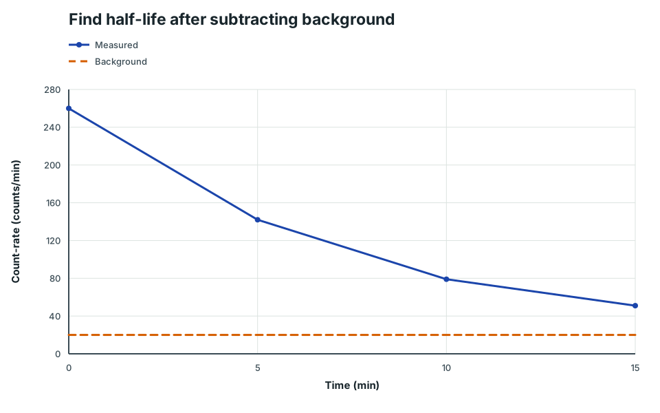
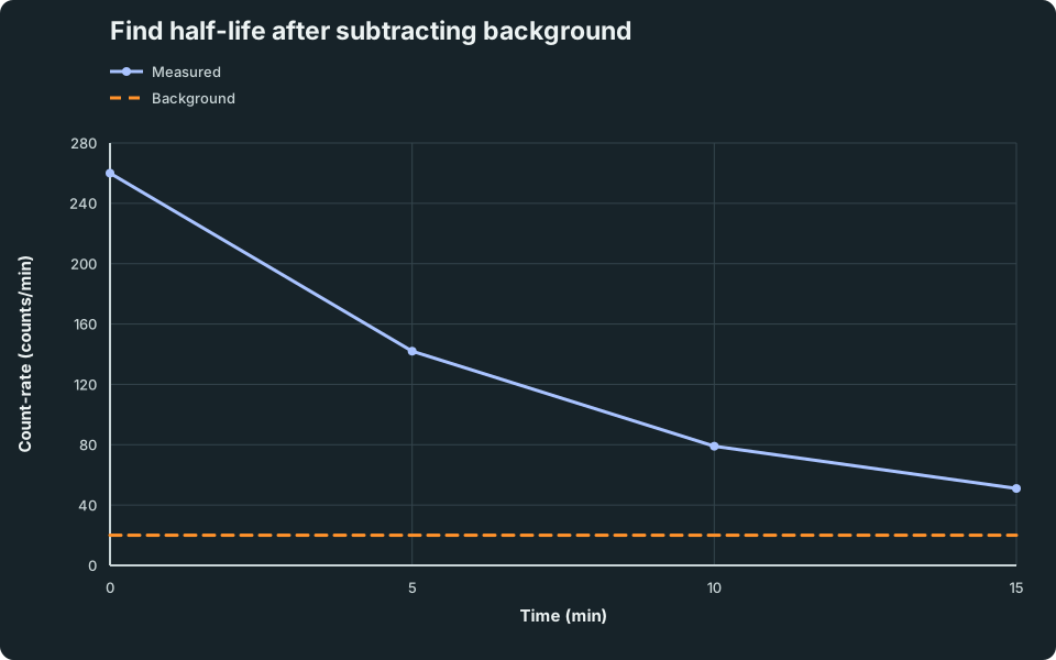
View figure data

Values and uncertainty for Find half-life after subtracting background

Series	Time (min)	Time uncertainty	Count-rate (counts/min)	Count-rate uncertainty
Measured	0		260
Measured	5		142
Measured	10		79
Measured	15		51
Background	0		20
Background	15		20

Values and uncertainty for Find half-life after subtracting background

Series	Time (min)	Time uncertainty	Count-rate (counts/min)	Count-rate uncertainty
Measured	0		260
Measured	5		142
Measured	10		79
Measured	15		51
Background	0		20
Background	15		20

Guided practice 3

Find a halving interval

About 6 min

Problem

Use the observations in the plot or its data table. Find the corrected rates at 0 and 5 minutes, then estimate the half-life using these and the later readings.

Try this before viewing the solution

Corrected rate at 0 min (counts/min)

Corrected rate at 5 min (counts/min)

Estimated half-life (min)

Check my attempt

Hints

Hint 1: source contribution

Subtract the same background rate from every observation.

Hint 2: fractional change

Compare each corrected rate with half the preceding corrected rate. Small fluctuations need not give exact halves.

View solution step by step

1. Correct every observation

   Method

   Subtract 20 counts/min from each raw rate.

   Reason

   Background does not decay with this source.

   Working

   The corrected rates are 240, 122, 59 and 31 counts/min.

2. Compare fractional changes

   Method

   Look for approximately equal time intervals for halving.

   Reason

   Random readings need not halve exactly.

   Working

   240 → about 120 → about 60 → about 30 at five-minute intervals gives an estimated half-life of about 5 min.

Apply the method independently

A second illustrative record uses one-minute counts at fixed geometry. Background is 30 counts/min.

Initial source count-rate (counts/min)

Half-life (min)

Fraction remaining at 12 min (decimal)

Check my attempt

Repair a first error

A learner writes: “The raw count-rate starts at 350, so after one half-life it is 175. I then subtract background.” Identify the first incorrect operation and find the expected raw reading after one half-life.

First incorrect operation

Halving the raw count-rateSubtracting background at all

Expected raw count-rate (counts/min)

Check my attempt

Practice and next step

Use the Radioactivity topic check for focused practice and feedback. Then continue to Applications, hazards and protection.