The Maxwell–Boltzmann distribution
Explore the Maxwell–Boltzmann speed distribution, compare characteristic speeds and explain how temperature changes the distribution.
Offline pages
Saved on this device only. Connect at least once every 30 days to confirm Premium. Sign-out or a change of account removes saved copies.
On this page
You stopped at:
ContinueMolecules at one temperature have a range of speeds. A distribution describes how much of the population lies in each speed interval; one characteristic speed cannot do that job. Here you will connect velocity-state counting to the shape of the Maxwell–Boltzmann curve, read areas as probabilities and distinguish its peak, mean and rms speed.
At a glance
- Prerequisites: Boltzmann factor, kinetic energy, basic calculus.
- Outcomes: use the MB speed distribution and extract vₘₚ, v bar, and vᵣₘₛ.
- Key result:
f(v) = 4π v²(m/(2π kBT))^(3/2)e^(-mv²/(2kBT)).
- Common trap: treating f(v) as dimensionless; it is a probability density in speed.
Count states in velocity space
For a dilute, non-relativistic classical gas at equilibrium, measure velocity relative to the gas’s mean motion. For one species of molecular mass m and no bulk flow:
- Translational kinetic energy: E = (1/2)mv².
- State counting in velocity space contributes a factor 4π v².
- Occupation probability contributes the Boltzmann weight e^(-E/(kBT)) (see UY1: the Boltzmann distribution).
Convention: f(v)dv is probability of speed in [v,v + dv].
Physical interpretation (what the distribution and parameters mean):
- f(v) is a probability density: f(v) dv gives the probability in a small interval of width dv near v. A single exact speed has zero probability in this continuous model.
- The exponential e^(-mv²/(2kBT)) says large kinetic energies are suppressed when they exceed the thermal scale kBT.
- The factor v² is geometric: in 3D there are many more velocity states with radius v than near v = 0 (a spherical-shell counting effect in velocity space).
- The natural thermal speed scale is vₜₕ∼ square root of (kBT/m): hotter means broader distribution; heavier means narrower.
Build and interpret the speed density
Derivation spine (why this form appears):
- In equilibrium, the probability of a microstate with kinetic energy E = 1/2 mv² is weighted by the Boltzmann factor e^(-E/(kBT)).
- Velocity components are independent and isotropic, giving a 3D Gaussian in (vₓ,vy,vz):
f(vₓ) ∝ e^(-mvₓ²/(2kBT)) and similarly for y,z.
- Converting from components to speed introduces the Jacobian factor 4π v² (surface area of a sphere in velocity space).
Combine state counting and Boltzmann factor:
Normalize with ∫₀^∞ f(v) dv = 1 to get
An area, not a height, gives a fraction of the gas: Pr(a ≤ v ≤ b) = ∫ₐ^b f(v) dv. For a narrow interval on which the density changes little, this is approximately f(v)Δ v. A histogram bar represents a finite interval even if an instrument labels it with one central speed. The density of one velocity component can peak at zero while the speed density peaks above zero: they are different variables and count different sets of states.
Compare two temperatures on one speed scale
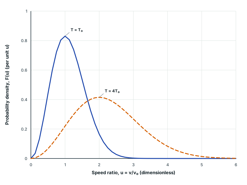
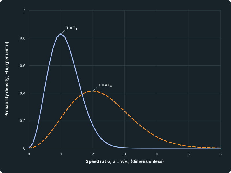
Let v₀ = square root of (2kBT₀/m) and u = v/v₀. Keep this reference speed fixed when comparing T₀ and 4T₀. The plotted density F(u) = v₀ f(v₀u) is per unit u, so its area gives probability just as f(v) dv does.
Heating stretches a speed distribution and lowers its peak
The horizontal coordinate is u = v/v₀ and the vertical coordinate is probability density per unit u. The solid T₀ curve peaks at u = 1; the dashed 4T₀ curve peaks at u = 2 with half the height. Both full distributions integrate to one, with tails beyond the finite plotted range.
Scroll across the figure to read all labels.
View figure data
| Speed ratio, u = v/v₀ (dimensionless) | T = T₀ | T = 4T₀ |
|---|---|---|
| 0.000 | 0.000e+00 | 0.000000 |
| 0.125 | 3.472e-02 | 0.004391 |
| 0.250 | 1.325e-01 | 0.017358 |
| 0.375 | 2.757e-01 | 0.038299 |
| 0.500 | 4.394e-01 | 0.066251 |
| 0.625 | 5.965e-01 | 0.099941 |
| 0.750 | 7.233e-01 | 0.137862 |
| 0.875 | 8.035e-01 | 0.178355 |
| 1.000 | 8.302e-01 | 0.219696 |
| 1.125 | 8.056e-01 | 0.260188 |
| 1.250 | 7.391e-01 | 0.298242 |
| 1.375 | 6.442e-01 | 0.332452 |
| 1.500 | 5.352e-01 | 0.361649 |
| 1.625 | 4.250e-01 | 0.384946 |
| 1.750 | 3.232e-01 | 0.401758 |
| 1.875 | 2.359e-01 | 0.411807 |
| 2.000 | 1.653e-01 | 0.415107 |
| 2.125 | 1.115e-01 | 0.411941 |
| 2.250 | 7.232e-02 | 0.402815 |
| 2.375 | 4.520e-02 | 0.388418 |
| 2.500 | 2.723e-02 | 0.369564 |
| 2.625 | 1.582e-02 | 0.347147 |
| 2.750 | 8.867e-03 | 0.322086 |
| 2.875 | 4.798e-03 | 0.295285 |
| 3.000 | 2.507e-03 | 0.267593 |
| 3.125 | 1.265e-03 | 0.239776 |
| 3.250 | 6.166e-04 | 0.212497 |
| 3.375 | 2.905e-04 | 0.186304 |
| 3.500 | 1.323e-04 | 0.161623 |
| 3.625 | 5.824e-05 | 0.138767 |
| 3.750 | 2.479e-05 | 0.117935 |
| 3.875 | 1.020e-05 | 0.099229 |
| 4.000 | 4.063e-06 | 0.082668 |
| 4.125 | 1.565e-06 | 0.068202 |
| 4.250 | 5.830e-07 | 0.055727 |
| 4.375 | 2.100e-07 | 0.045101 |
| 4.500 | 7.300e-08 | 0.036158 |
| 4.625 | 2.500e-08 | 0.028718 |
| 4.750 | 8.000e-09 | 0.022599 |
| 4.875 | 3.000e-09 | 0.017621 |
| 5.000 | 1.000e-09 | 0.013614 |
| 5.125 | 0.000e+00 | 0.010424 |
| 5.250 | 0.000e+00 | 0.007910 |
| 5.375 | 0.000e+00 | 0.005948 |
| 5.500 | 0.000e+00 | 0.004434 |
| 5.625 | 0.000e+00 | 0.003276 |
| 5.750 | 0.000e+00 | 0.002399 |
| 5.875 | 0.000e+00 | 0.001742 |
| 6.000 | 0.000e+00 | 0.001253 |
For fixed mass, raising temperature by a factor a gives f_aT(v) = a^(-1/2)fT(v/square root of a). At four times the temperature the speed axis stretches by two and the peak height halves; the full area stays one. The graph shows a finite speed range, not the entire tail. Changing the horizontal scale also changes density height, so compare heights only with the same variable and units.
Characteristic speeds:
Therefore
Consistency check (connects back to kinetic temperature):
agreeing with UY1: root-mean-square speed of the gas particles and the kinetic definition of T in UY1: concept of kinetic temperature.
Units check:
- Since f(v)dv is dimensionless, [f(v)] = (m s⁻¹)⁻¹ = s m⁻¹.
Physical sanity checks:
- f(0) = 0 because of v² state-counting factor.
- As v → ∞, exponential decay forces f(v) → 0.
- Higher T shifts the peak to larger v and broadens the curve.
Limit checks:
- As T → 0, the distribution collapses toward v = 0 (in the classical model).
- For fixed T, increasing m makes the distribution narrower (heavier molecules have smaller typical speeds).
- f(v) is a probability density, with units of inverse speed. Probability is the area over a speed interval.
- Speed is non-negative. The range -∞ to ∞ belongs to a signed velocity component, rather than speed.
- Pair molecular mass m with kB, or molar mass M with R.
Characteristic speeds of argon
Worked example 1
Three characteristic speeds
Problem
Show full solution
Use molar rather than molecular mass
Method
Replace kB/m by R/M in each speed formula.Reason
The given mass is per mole. Since R = NAkB and M = NAm, their ratio preserves the molecular formula.Working
Answer
vₘₚ = square root of (2RT/M) ≈ 353 m s⁻¹,v bar = square root of (8RT/(π M)) ≈ 398 m s⁻¹,vᵣₘₛ = square root of (3RT/M) ≈ 433 m s⁻¹.Compare the three results
Working
Answer
vₘₚ ≈ 353 m s⁻¹, v bar ≈ 398 m s⁻¹ and vᵣₘₛ ≈ 433 m s⁻¹. Their ordering matches vᵣₘₛ > v bar > vₘₚ; the square roots of RT/M have speed units.
Practice set
Check your understanding 1
Use the Maxwell–Boltzmann formulas to show that vᵣₘₛ > v bar for the same gas at a positive temperature.
Show hint
Show answer
Check your understanding 2
For a fixed gas, how does the most probable speed change when absolute temperature quadruples?
Show hint
Show answer
Check your understanding 3
For a fixed gas, temperature rises from 250 K to 500 K. By what factor does the speed at the distribution peak change?
Show hint
The peak occurs at vₘₚ, not at the mean speed.
Show answer
The peak speed increases by square root of (500/250) = square root of 2 ≈ 1.41. This is a shift along the speed axis, not a factor for the peak height.
Read a finite speed interval
Guided practice 2
Turn density into a fraction of the gas
Problem
A classical equilibrium gas contains 10⁶ molecules. At temperature T₀, its speed density is approximately constant at f_T₀(500 m s⁻¹) = 1.20 × 10⁻³ s m⁻¹ across a narrow interval of width 20.0 m s⁻¹ centred there. Estimate the interval probability and expected number of molecules. Then find f_4T₀(1000 m s⁻¹) for the same gas. Explain why the density value alone is not the interval probability.
Work through the model, then compare your reasoning
Hints
Hint 1
Check the model
Track the units of height and width. For the temperature change, use the same speed axis and the corresponding doubled speed.Show solution step by step
Read an area as probability
Method
Use the narrow-bin approximation.Reason
The density has inverse-speed units.Working
Answer
p ≈ fΔ v = 0.0240, so the expected count is 10⁶p = 24000. This is an expectation, not a guarantee of exactly that many particles in a fluctuating sample.
Keep normalisation when temperature changes
Method
Apply f_4T₀(v) = (1/2)f_T₀(v/2).Reason
A doubled horizontal scale requires a halved density at the corresponding coordinate.Working
Answer
f_4T₀(1000) = 6.00 × 10⁻⁴ s m⁻¹. Doubling the corresponding bin width to 40.0 m s⁻¹ would keep its probability approximately 0.0240. The probability at one exact mathematical speed is zero; an instrument interval has a finite width.
Compare unequal measurement bins
Check your understanding 4
For one speed distribution, the density is nearly constant at 9.0 × 10⁻⁴ s m⁻¹ across a 10 m/s bin centred near 200 m/s, and 5.0 × 10⁻⁴ s m⁻¹ across a 30 m/s bin centred near 500 m/s. Estimate each bin’s probability and decide which contains the larger expected fraction. A student chooses the taller density value and says a meter displaying “500 m/s” is impossible because one exact speed has probability zero. Evaluate both statements.
Show answer
The approximate fractions are (9.0 × 10⁻⁴)(10) = 0.0090 and (5.0 × 10⁻⁴)(30) = 0.015. The wider second bin contains more probability despite its lower density. If density varies appreciably, use the integral over each bin instead. A rounded meter reading represents a finite resolution interval, so it can have nonzero probability; it is not an infinitely precise mathematical point. Neither a bin height nor the most probable speed is the fraction of gas in an interval.
What to keep
A speed-density height has inverse-speed units; probability is an area. The v² factor counts velocity states in three dimensions. Peak, mean and rms speed differ, and temperature changes both horizontal scale and density height while preserving the full probability.
Spotted an error? Report a correction
Syllabus and review details
No official syllabus alignment is listed for this lesson.