Quantities & Measurement

• Uncertainty (instrument): analogue ≈ ± 1/2 smallest division; digital ≈ ± 1 in the last displayed digit (unless stated).
• A ± B: Add absolute uncertainties ( Δ A + Δ B)
• A × B or A/B: Add percentage uncertainties ( (Δ A)/A% + (Δ B)/B%)
• Aⁿ: Multiply % uncertainty by |n| ( n × (Δ A)/A%)
• Vectors: Rₓ = R cos θ, R_y = R sin θ (Check quadrant signs!)
• Log graphs: for y = kxⁿ, ln y = ln k + n ln x (gradient = n, intercept = ln k).

• Homogeneity: A valid physical equation must have the same base units on both sides.
• Systematic Error: A consistent deviation from the true value (e.g., zero error); affects accuracy.
• Random Error: Unpredictable fluctuations around the true value; affects precision; reduced by averaging.
• Accuracy: Closeness to the true value.
• Precision: Closeness of repeated readings to each other (small spread).
• Absolute Uncertainty: The actual error margin (e.g., ± 0.1 cm).
• Fractional/Percentage Uncertainty: The error margin relative to the value (e.g., ± 2%).

Uncertainty workflow

1. Write the formula for the derived quantity.
2. Convert all measurements to consistent units.
3. Combine uncertainties (absolute for +/−, % for ×/÷/powers).
4. Round the final value to match the uncertainty (uncertainty sets the precision).

Graph workflow

1. Label axes as Quantity / Unit, choose a sensible scale, plot neat points.
2. Draw a best-fit line/curve (don’t join dot-to-dot).
3. Use a large triangle for gradient; state units.
4. Don’t force the origin unless the physics requires it; interpret intercepts as offsets/systematic error.

In A Level practicals, graphs are not just “presentation”: they help you spot systematic error and extract constants from gradients.

Best-fit line + intercept (systematic error check)

If a model predicts direct proportionality but the best-fit line has a significant non-zero intercept, investigate a zero error, constant offset, or an incomplete model. The intercept is evidence to interpret, not proof of one particular error.

Extension against force (example practical data)

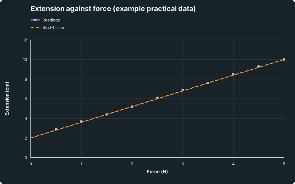
Extension readings plotted against force with a non-zero best-fit intercept. The intercept may indicate an offset or a limitation in the assumed model.

Scroll across the graph to read all labels.

Open full-size graph

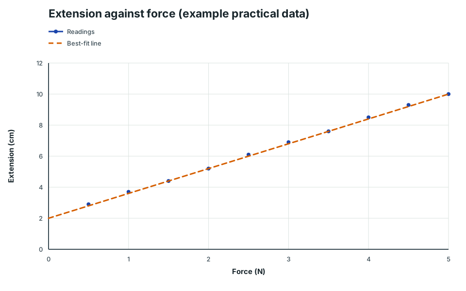
View figure data

Values and uncertainty for Extension against force (example practical data)

Series	Force (N)	Force uncertainty	Extension (cm)	Extension uncertainty
Readings	0.5		2.9
Readings	1		3.7
Readings	1.5		4.4
Readings	2		5.2
Readings	2.5		6.1
Readings	3		6.9
Readings	3.5		7.6
Readings	4		8.5
Readings	4.5		9.3
Readings	5		10
Best-fit line	0		2
Best-fit line	5		10

Values and uncertainty for Extension against force (example practical data)

Series	Force (N)	Force uncertainty	Extension (cm)	Extension uncertainty
Readings	0.5		2.9
Readings	1		3.7
Readings	1.5		4.4
Readings	2		5.2
Readings	2.5		6.1
Readings	3		6.9
Readings	3.5		7.6
Readings	4		8.5
Readings	4.5		9.3
Readings	5		10
Best-fit line	0		2
Best-fit line	5		10

Which measurement dominates the uncertainty?

For a derived quantity, a quick “uncertainty budget” helps you decide what to improve.

Example: density of a cylinder, ρ = m/(π r² L).

(Δ ρ)/ρ% ≈ (Δ m)/m% + 2(Δ r)/r% + (Δ L)/L%

1. Homogeneity ≠ Correctness: An equation can be dimensionally correct but physically wrong (e.g., missing a constant like 1/2 or 2π).
2. Adding % Errors: You can ONLY add percentage/fractional uncertainties for multiplication and division. For addition/subtraction, you MUST add absolute uncertainties.
3. Significant Figures: The uncertainty determines the precision of the final answer. E.g., if uncertainty is ± 0.1, don’t write 2.345.
4. Vector Signs: When resolving forces, explicitly define positive directions (e.g., Up/Right = +ve). Gravity is usually negative in vertical motion.
5. Log Graphs: For y = kxⁿ, plotting ln y vs ln x gives a straight line with gradient n. Don’t confuse log (base 10) with ln (base e).