Uncertainty
Key idea: Learn how to estimate measurement uncertainties, distinguish random vs systematic errors, and propagate uncertainties for +, −, ×, ÷ and powers.
Continue where you stopped
The core idea
On this page
Learning objectives
- Assess random, systematic and propagated uncertainties.
These “propagation rules” are a fast, conservative way to estimate uncertainties. In university labs you’ll also meet statistical approaches (standard deviation, standard error), but the logic here is still a useful baseline.
1. Definitions (Must Know)
- Error: the difference between a measured value and the true value (true value is usually unknown).
- Uncertainty, Δ x: an estimate of the possible range of values around a measurement x.
- Absolute uncertainty, Δ x: uncertainty written in the same unit as x (e.g. 2.50 ± 0.05 m).
- Fractional uncertainty: (Δ x)/x (no unit).
- Percentage uncertainty: (Δ x)/x × 100%.
- Random error: unpredictable variation between repeated readings; causes scatter. Repeats reveal the spread, and averaging reduces the random contribution to the mean.
- Systematic error: consistent bias (e.g. zero error, calibration error); affects accuracy; not reduced by averaging.
- Precision: how close repeated readings are to each other (small scatter).
- Accuracy: how close a measurement is to the true value.
2. Key Ideas (What Earns Marks)
- Quote readings with sensible uncertainty:
- analogue scale: ± half the smallest division,
- digital reading: typically ± 1 in the last displayed digit (unless stated otherwise),
- repeated readings: random uncertainty ≈ half the range.
- For a derived quantity, propagate uncertainties using the standard A Level rules (worst-case approach):
- If Y = a ± b: Δ Y = Δ a + Δ b
- If Y = ab or Y = a/b: (Δ Y)/Y = (Δ a)/a + (Δ b)/b
- If Y = aⁿ: (Δ Y)/Y = |n| (Δ a)/a
- If the expression is awkward, use numerical substitution (max–min):
- compute Yₘₐₓ and Yₘᵢₙ using the extreme values,
- then Δ Y ≈ (Yₘₐₓ-Yₘᵢₙ)/2.
- Quote the final answer so the value and uncertainty match:
- uncertainty: usually 1 s.f. (2 s.f. is common if it starts with 1 or 2),
- value: same decimal place as the uncertainty.
3. Detailed Explanations
A. Estimating uncertainty in a measurement
Use the information the question gives you.
Common defaults:
- Analogue scale: uncertainty ≈ ± half the smallest division.
- Digital display: uncertainty ≈ ± 1 in the last displayed digit.
- Repeats (random uncertainty): uncertainty ≈ half range.
Example (percentage given): If a timer is specified as ± 0.1% and you measure t = 638.5 ms, then Δ t = 0.001 × 638.5 ≈ 0.6 ms So quote t = 638.5 ± 0.6 ms.
B. Random vs systematic errors (what examiners want)
- Random error mainly affects precision. Repeating reveals its size; averaging reduces its effect on the mean but does not remove the scatter in the measurements.
- Systematic error mainly affects accuracy. Averaging does not remove it (you must correct/calibrate).
If you see “zero error”, “calibration error”, “parallax always in the same direction”, treat it as systematic.
C. Propagating uncertainties: + and − (absolute uncertainties)
If Y = a + b or Y = a - b, add absolute uncertainties: Δ Y = Δ a + Δ b
Reason: you are estimating a worst-case uncertainty range.
D. Propagating uncertainties: × and ÷ (fractional/percentage uncertainties)
If Y = ab or Y = a/b, add fractional uncertainties: (Δ Y)/Y = (Δ a)/a + (Δ b)/b
You can do this in percentages as well: %Δ Y = %Δ a + %Δ b
E. Powers (including roots)
If Y = aⁿ: (Δ Y)/Y = |n|(Δ a)/a
Examples:
- Y = a²: percentage uncertainty doubles.
- Y = square root of a = a^(1/2): percentage uncertainty halves.
F. Uncertainty budget (spot the dominant term)
A quick way to decide what to improve is to break the result into percentage contributions from each measurement.
Example (simple pendulum): g = 4π²L/T² So, %Δ g ≈ %Δ L + 2%Δ T
Data table
| Category | Contribution |
|---|---|
| Length, L | 0 |
| Time, T (×2) | 2 |
G. Numerical substitution (max–min method)
Use this when the expression is awkward.
Workflow:
- Compute the best estimate Y using best values.
- Compute Yₘₐₓ using values that make Y as large as possible.
- Compute Yₘᵢₙ using values that make Y as small as possible.
- Estimate: Δ Y ≈ (Yₘₐₓ-Yₘᵢₙ)/2 and %Δ Y ≈ 100% × (Δ Y)/Y.
4. Common Mistakes
- Adding percentage uncertainties for addition/subtraction (wrong). For + and -, add absolute uncertainties.
- Adding absolute uncertainties for multiplication/division (usually wrong). For × and ÷, add fractional/percentage uncertainties.
- Rounding too early (causes noticeable drift in uncertainty questions). Keep guard digits until the end.
- Quoting an answer with inconsistent precision (e.g. 2.345 ± 0.1). Match decimal places.
- Treating a systematic error as “reduced by repeats”.
5. Exam Tips
- Write the rule you are using before you substitute (it signals method marks).
- If one measurement has a much larger percentage uncertainty, it usually dominates the final uncertainty.
- If you are asked for an “uncertainty in Y”, state whether you are giving absolute or percentage.
- A good final line format is:
- Y = (value ± Δ Y) unit
- or Y = value unit (± percentage)
- Related: Dimensional Analysis (unit checks) and the A Level Practical Hub (evaluation + uncertainties in Paper 4).
Practical Lab
Use this workflow-first lab if you want the Paper 4 version of this topic rather than another static summary:
Practical Lab: Uncertainty & Error Propagation
Work through instrument readings, repeated data, propagation, and final reporting with an exam-style uncertainty workflow.
- Absolute vs Percentage Uncertainty
- Repeated-Reading Estimate
- Propagation Rules
- Final Answer Reporting
6. Worked Examples
Modelled example 1
Addition/subtraction (absolute uncertainty)
Problem
Study the worked solution
Find the best estimate
Method
Add measured values.Reason
The derived length is defined by addition.Working
L = 12.4 + 8.2 = 20.6 cmPropagate absolute uncertainties
Method
Add the absolute uncertainties.Reason
The conservative addition/subtraction rule operates in the quantity’s units.Working
Δ L = 0.1 + 0.1 = 0.2 cmReport consistently
Method
State 20.6±0.2 cm.Reason
Value and absolute uncertainty share units and decimal place.Working
L = 20.6±0.2 cm.
Guided practice 2
Multiplication/division (percentage uncertainty)
Problem
Try this before viewing the solution
Hints
Hint 1: division uses relative uncertainty
View solution step by step
Find resistance
Method
Calculate the best estimate.Reason
R = V/I.Working
R = 10.0/1.3 = 7.7 ΩAdd percentage uncertainties
Method
Combine 3.0% and approximately 15%.Reason
For division, conservative fractional uncertainties add.Working
%Δ R = 3.0% + 15% = 18%Convert back to absolute
Method
Obtain approximately 1.4 Ω.Reason
The final result is reported in ohms.Working
Δ R = 0.18(7.7) = 1.4 Ω, R = 7.7±1.4 Ω
Common misconception 3
Power rule (common in Mechanics)
Learner claim
Try this before viewing the solution
View solution step by step
Find height percentage uncertainty
Method
Divide absolute uncertainty by value.Reason
Power rules act on fractional or percentage uncertainty.Working
%Δ h = (0.01/2.00)100% = 0.5%Apply the exponent
Method
Multiply by 1/2.Reason
For v ∝ h^(1/2), the relative uncertainty factor is the exponent magnitude.Working
%Δ v = (1/2)(0.5%) = 0.25%
Examiner practice 4
Speed from distance/time
Examination question
Try this before viewing the solution
View solution step by step
Find speed
1 markMethod
Divide distance by time.Reason
v = d/t.Working
v = 100.00/9.63 = 10.38 m s⁻¹Find input percentages
1 markMethod
Obtain 0.01% and 0.10%.Reason
Each is absolute uncertainty divided by its value.Working
%Δ d = 0.01%; %Δ t ≈ 0.10%.Propagate
1 markMethod
Add to approximately 0.11%.Reason
Speed is a quotient.Working
%Δ v ≈ 0.11%.Report absolute uncertainty
1 markMethod
State 10.38±0.01 m s⁻¹.Reason
0.0011(10.38) ≈ 0.01 m s⁻¹.Working
v ≈ 10.38±0.01 m s⁻¹.
Self-mark with the mark scheme
Compare your response with each mark point. Select a point only when your response contains that evidence.
Self-mark estimate, percentages, propagation and reported result.
Challenge 5
Uncertainty in gradient (max–min method)
Independent graph transfer
Try this before viewing the solution
Hints
Hint 1: choose opposite uncertainty-box corners
View solution step by step
Construct best and extreme gradients
Method
Calculate the best gradient, then the steepest and shallowest acceptable lines.Reason
The uncertainty boxes bound plausible endpoint positions, and half the extreme-gradient range estimates gradient uncertainty.Working
Best estimate gradient: R = (Δ V)/(Δ I) = (8.40-2.10)/(0.80-0.20) = 6.30/0.60 = 10.5 Ω
To estimate uncertainty, find extreme gradients.
Maximum gradient: maximise numerator and minimise denominator. Δ Vₘₐₓ = (8.40 + 0.05)-(2.10-0.05) = 6.40 V Δ Iₘᵢₙ = (0.80-0.01)-(0.20 + 0.01) = 0.58 A Rₘₐₓ ≈ 6.40/0.58 ≈ 11.0 Ω
Minimum gradient: minimise numerator and maximise denominator. Δ Vₘᵢₙ = (8.40-0.05)-(2.10 + 0.05) = 6.20 V Δ Iₘₐₓ = (0.80 + 0.01)-(0.20-0.01) = 0.62 A Rₘᵢₙ ≈ 6.20/0.62 = 10.0 Ω
So, Δ R ≈ (Rₘₐₓ-Rₘᵢₙ)/2 = (11.0-10.0)/2 = 0.5 Ω
Final: R ≈ 10.5 ± 0.5 Ω
Max–min gradients from the same two points
Best-fit line and the steepest/shallowest plausible gradients based on the stated uncertainties.
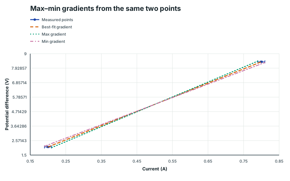
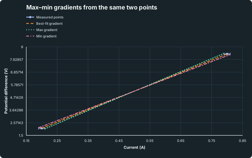
Inspect either measured point and its uncertainty, then compare it with the steepest and shallowest acceptable gradients.
Optional interaction loads only after you choose Explore graph.
The error bars show each stated uncertainty box. The steepest acceptable line joins (0.21 A, 2.05 V) to (0.79 A, 8.45 V); the shallowest joins (0.19 A, 2.15 V) to (0.81 A, 8.35 V). Open full-size graphView figure data
Values and uncertainty for Max–min gradients from the same two points Series Current (A) Current uncertainty Potential difference (V) Potential difference uncertainty Measured points 0.2 0.01 2.1 0.05 Measured points 0.8 0.01 8.4 0.05 Best-fit gradient 0.2 2.1 Best-fit gradient 0.8 8.4 Max gradient 0.21 2.05 Max gradient 0.79 8.45 Min gradient 0.19 2.15 Min gradient 0.81 8.35
7. Mind Stretchers
Mind stretcher 1: Numerical substitution (max–min)Extension
A student finds density from ρ = m/V where m = 52.3 ± 0.1 g and V = 19.5 ± 0.5 cm³. Use max–min to estimate ρ and Δ ρ.
Show Answer
Best estimate: ρ = 52.3/19.5 = 2.68 g cm⁻³
Extremes:
- ρₘₐₓ = 52.4/19.0 = 2.76
- ρₘᵢₙ = 52.2/20.0 = 2.61
So, Δ ρ ≈ (2.76-2.61)/2 = 0.075 g cm⁻³ ≈ 0.08 g cm⁻³
Final: ρ ≈ 2.68 ± 0.08 g cm⁻³
If you need SI units: 1 g cm⁻³ = (10⁻³ kg)/(10⁻⁶ m³) = 10³ kg m⁻³ So, ρ ≈ (2.68 ± 0.08) × 10³ kg m⁻³ ≈ (2680 ± 80) kg m⁻³
Mind stretcher 2: Uncertainty in g from a pendulum (power rule + multiplication)Extension
For a simple pendulum, g = 4π²L/T².
If L = 0.800 ± 0.002 m and T = 1.80 ± 0.02 s, estimate the percentage uncertainty in g.
Show Answer
%Δ g = %Δ L + 2%Δ T
%Δ L = 0.002/0.800 × 100% = 0.25% %Δ T = 0.02/1.80 × 100% ≈ 1.1%
So, %Δ g ≈ 0.25% + 2(1.1%) ≈ 2.5%
Mind stretcher 3: Optional (Enrichment)Extension
A. Standard deviation (beyond syllabus)
In the A Level syllabus, you do not need a rigorous statistical treatment.
If you meet standard deviation in other contexts: it is a measure of the spread of repeated readings around the mean. It is useful when you have many repeats and want a more formal uncertainty estimate than “half range”.
Continue with the next resource in this course.
Course and syllabus information
- Course
- GCE A-Level H2 Physics
- Edition
- GCE A-Level H2 Physics 2027