Kinematics

Useful components: uₓ = u cos θ, u_y = u sin θ.

Max height: when v_y = 0.

Same launch and landing height (no air resistance):

• time of flight: T = 2u_y/g
• max height: H = u_y²/2g
• range: R = uₓ T = (u² sin 2θ)/g

SUVAT (1D, constant acceleration only)

• v = u + at
• s = ut + (1/2)at²
• v² = u² + 2as
• s = (1/2)(u + v)t

• Displacement: Change in position from the initial point to the final point, with direction.
• Velocity: Rate of change of displacement.
• Acceleration: Rate of change of velocity.
• Projectile motion (ideal model): Motion with uniform velocity in one direction and uniform acceleration in a perpendicular direction. Near Earth, this is usually modelled with air resistance neglected.
• Weight: The force experienced by a mass in a gravitational field, W = mg near Earth’s surface.
• Gravitational potential energy change: For the mass–Earth system in a uniform field, Δ Eₚ = mgΔ h.
• Terminal velocity: Constant downward velocity reached when drag balances weight, so the resultant force and acceleration are zero.

Projectile motion (component method)

1. Choose axes and state sign convention (e.g., up is +).
2. Resolve initial velocity: uₓ = u cos θ, u_y = u sin θ.
3. Write x-motion (uniform): x = uₓt.
4. Write y-motion (uniform acceleration): y = u_yt-(1/2)gt² and v_y = u_y-gt.
5. Use the same time t to connect x and y, then solve.

Graph method (1D)

1. State what the gradient/area represents (units matter).
2. Use a large triangle for gradients; split area into shapes.
3. For a curve, use a tangent for instantaneous gradient.

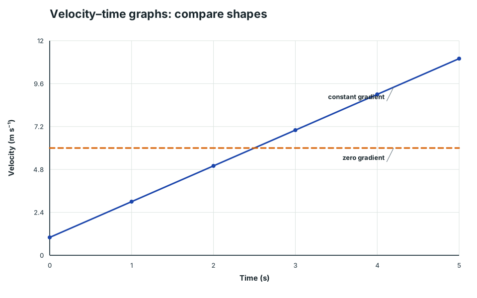
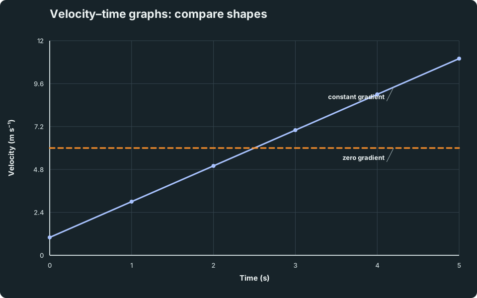
Velocity–time: gradient is acceleration

Velocity–time graphs: compare shapes

Two velocity–time series from zero to five seconds. One rises from one to eleven metres per second with constant gradient two metres per second squared. The other remains at six metres per second.

View figure data

Values for Velocity–time graphs: compare shapes

Time (s)	Constant acceleration, a = 2 m s⁻²	Constant velocity, a = 0 m s⁻²
0	1	6
1	3	6
2	5	6
3	7	6
4	9	6
5	11	6

Values for Velocity–time graphs: compare shapes

Time (s)	Constant acceleration, a = 2 m s⁻²	Constant velocity, a = 0 m s⁻²
0	1	6
1	3	6
2	5	6
3	7	6
4	9	6
5	11	6

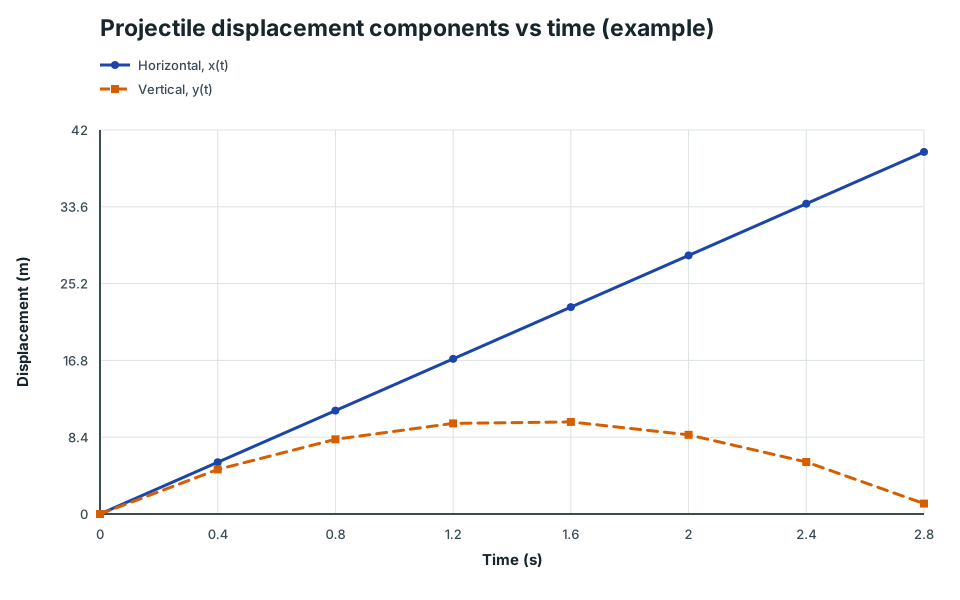
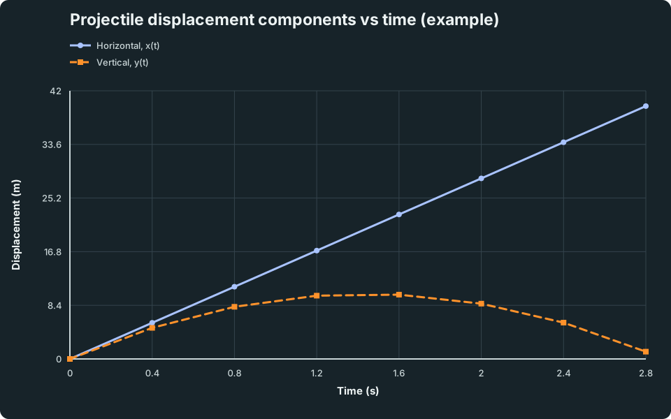
Projectile components share the same time

This plot uses a single time axis to show the key idea: x motion is uniform while y motion is uniformly accelerated.

Projectile displacement components vs time (example)

Horizontal displacement increases linearly with time; vertical displacement rises then falls back to zero.

Scroll across the graph to read all labels.

Open full-size graph

View figure data

Values for Projectile displacement components vs time (example)

Time (s)	Horizontal, x(t)	Vertical, y(t)
0	0	0
0.4	5.66	4.87
0.8	11.31	8.17
1.2	16.97	9.91
1.6	22.63	10.07
2	28.28	8.66
2.4	33.94	5.69
2.8	39.6	1.14

Values for Projectile displacement components vs time (example)

Time (s)	Horizontal, x(t)	Vertical, y(t)
0	0	0
0.4	5.66	4.87
0.8	11.31	8.17
1.2	16.97	9.91
1.6	22.63	10.07
2	28.28	8.66
2.4	33.94	5.69
2.8	39.6	1.14

1. Independence of Components: Horizontal motion does not affect vertical motion. They are linked only by time (t).
2. Sign Convention: Pick a direction (usually Up) as positive. Then a = -9.81. If you swap mid-question, you will get math errors.
3. Top of Trajectory: At max height, velocity is not zero; the vertical component v_y = 0, but horizontal vₓ is still there!
4. Air Resistance: In projectiles, we usually ignore it. If included, the path is no longer a perfect parabola (range and max height decrease).
5. Graph Gradients: On a displacement-time graph, a curve means changing velocity. On a velocity-time graph, a curve means non-uniform acceleration.
6. Terminal Velocity: Zero acceleration at terminal velocity does not mean zero velocity; it means constant velocity because drag equals weight.