Kinematics Graphs (A Level)
Key idea: Learn how to interpret distance–time, displacement–time, velocity–time and acceleration–time graphs using gradients, areas and tangents (A Level Physics).
Continue where you stopped
The core idea
On this page
Learning objectives
- Interpret position, displacement, velocity and acceleration using equations and graphs.
- Derive the uniformly accelerated motion equations from the definitions of velocity and acceleration.
- Derive and apply uniformly accelerated motion equations with a stated sign convention.
1. Definitions (Must Know)
A kinematics graph shows how a motion quantity changes with time.
Two graph skills that show up again and again:
- Gradient (slope):
gradient = Δy / Δx(units: “y-unit per x-unit”) - Area under a graph: add up areas of simple shapes (rectangles/triangles/trapeziums). Units: “y-unit × x-unit”.
A. Instantaneous value (tangent idea)
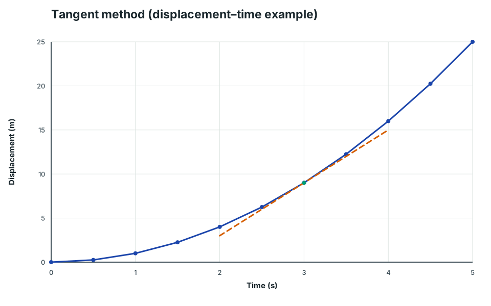
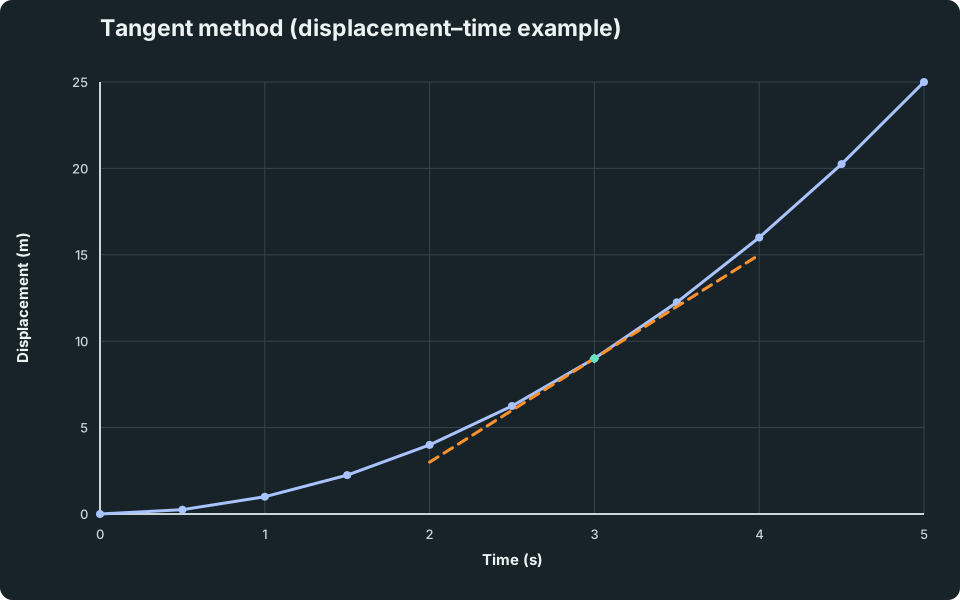
For a curved displacement–time graph, instantaneous velocity is found from the gradient of the tangent at that point. For a curved velocity–time graph, the tangent gradient gives instantaneous acceleration. The graph’s vertical coordinate itself is the instantaneous value of the quantity named on its vertical axis.
Tangent method (displacement–time example)
A curve s=t^2 with a tangent at t=3 s. The gradient of the tangent gives instantaneous velocity.
Scroll across the graph to read all labels.
View figure data
| Series | Time (s) | Time uncertainty | Displacement (m) | Displacement uncertainty |
|---|---|---|---|---|
| Curve: s = t² | 0 | 0 | ||
| Curve: s = t² | 0.5 | 0.25 | ||
| Curve: s = t² | 1 | 1 | ||
| Curve: s = t² | 1.5 | 2.25 | ||
| Curve: s = t² | 2 | 4 | ||
| Curve: s = t² | 2.5 | 6.25 | ||
| Curve: s = t² | 3 | 9 | ||
| Curve: s = t² | 3.5 | 12.25 | ||
| Curve: s = t² | 4 | 16 | ||
| Curve: s = t² | 4.5 | 20.25 | ||
| Curve: s = t² | 5 | 25 | ||
| Tangent at t = 3 s | 2 | 3 | ||
| Tangent at t = 3 s | 4 | 15 | ||
| Point at t = 3 s | 3 | 9 |
2. Key Ideas (What Earns Marks)
| Graph | Gradient tells you | Area tells you |
|---|---|---|
| Distance–time | speed (m s⁻¹) | (not usually used) |
| Displacement–time | velocity (m s⁻¹) | (not usually used) |
| Velocity–time | acceleration (m s⁻²) | displacement, s (m, signed) |
| Acceleration–time | (not usually used) | change in velocity, Δ v (m s⁻¹) |
- Sign matters for displacement and velocity. Decide your positive direction first.
On a velocity-time graph, gradient gives acceleration while area gives displacement. Swapping these two ideas usually costs all method marks in graph questions.
A negative gradient on a velocity–time graph means negative acceleration. The object slows down only when velocity and acceleration have opposite signs; if both are negative, its speed increases in the negative direction.
Interactive Concept Explorer: s-t, v-t, a-t Links
Use this explorer to stress-test your graph intuition across presets and marker positions:
- slope of s-t gives v
- slope of v-t gives a
- area under v-t gives displacement
Concept Explorer: Kinematics Graph Relationships
Switch graph-shape presets, move the time marker, and connect slope/area ideas across position-time, velocity-time, and acceleration-time graphs.
- Gradient Interpretation
- Signed Area
- Direction From Velocity
- Graph Translation
Explore the motion graphs in the Kinematics Graph Explorer.
3. Detailed Explanations
A. Distance–time graphs
- Distance never decreases.
- Horizontal line → object is stationary.
- Steeper gradient → higher speed.
- Curve → speed is changing (non-uniform speed).
B. Displacement–time graphs
- Displacement can be positive, negative, or zero (depends on your chosen origin and direction).
- Displacement can increase, decrease, or stay constant.
- Straight line → uniform velocity.
- Negative gradient → motion in the opposite direction.
- For a curve, the instantaneous velocity is the gradient of the tangent (A Level idea).
C. Velocity–time graphs
- Horizontal line → constant velocity.
- Straight line with positive gradient → uniform acceleration.
- Straight line with negative gradient → uniform negative acceleration. Whether the object speeds up or slows down depends on the velocity sign.
- Curve → acceleration is changing.
- Area under the graph → displacement (signed area).
- Total distance travelled → add areas using absolute values (treat areas below the axis as positive).
D. Acceleration–time graphs
- Area under the graph → change in velocity.
- A horizontal line above zero means constant positive acceleration; below zero means constant negative acceleration.
E. Relationship between the graphs (summary)
This schematic shows constant positive acceleration. It is not a universal set of shapes: the relationships between gradient and signed area are the transferable rule.
F. Deriving the SUVAT equations (constant acceleration)
If acceleration is constant, the velocity–time graph is a straight line, so:
- gradient gives acceleration: a = (v-u)/t ⇒ v = u + at
- area gives displacement: s = v_avgt = (1/2)(u + v)t
Substitute v = u + at into the average-velocity result:
s = ut + (1/2)at²
Eliminate t between v = u + at and s = (1/2)(u + v)t:
v² = u² + 2as
These equations apply only to straight-line motion with constant acceleration. Define the positive direction before substituting signed values for u, v, a and s.
4. Common Mistakes
- Mixing up distance vs displacement (sign matters for displacement).
- Forgetting that area below the time-axis is negative displacement (but still adds to distance).
- Finding a gradient using two points that are too close together (large percentage error).
- Calling every negative gradient “deceleration”. Compare the signs of velocity and acceleration before deciding whether speed decreases.
5. Exam Tips
- When asked for an instantaneous value on a curve, draw a tangent and use two well-separated points on the tangent.
- Always show units:
gradient of v–tism s⁻², and area underv–tism.
6. Worked Examples
Modelled example 1
Acceleration–time graph (area idea)
Problem
Study the worked solution
Translate graph area
Method
The signed area accumulated from the start gives the object’s velocity.Reason
Area under an acceleration–time graph is change in velocity, and the initial velocity is zero.Working
v(t) = 0 + signed area from 0 to tCompare the labelled points
Method
Point 2 has the largest speed.Reason
At point 2, the magnitude of the accumulated signed area—and therefore the velocity magnitude—is greatest.Working
largest |v| ↔ largest accumulated |area|
Guided practice 2
Average speed vs average velocity (out-and-back)
Problem
Try this before viewing the solution
Hints
Hint 1: use an arbitrary one-way distance
View solution step by step
Add the travel times
Method
The total time is 8d/15.Reason
Times add, while speeds cannot be averaged directly because the two equal distances take unequal times.Working
t = d/5.00 + d/3.00 = 8d/15Calculate average speed
Method
3.75 m s⁻¹.Reason
Average speed is total distance 2d divided by total time.Working
v bar _speed = 2d/(8d/15) = 3.75 m s⁻¹Calculate average velocity
Method
0 m s⁻¹.Reason
Returning to A makes the net displacement zero.Working
v bar = Δ s/Δ t = 0
Guided practice 3
Hare and tortoise (photo finish)
Problem
Try this before viewing the solution
Hints
Hint 1: match remaining times
View solution step by step
Find the hare's remaining distance
Method
The hare has 200 m left.Reason
It has completed 0.800 km of the 1.00 km course.Working
1.00-0.800 = 0.200 km = 200 mFind the hare's remaining time
Method
25.0 s.Reason
At constant speed, time is distance divided by speed.Working
t = 200/8.00 = 25.0 sMatch the tortoise distance
Method
The tortoise should be 5.00 m from the finish.Reason
It covers this distance during the hare’s remaining 25.0 s.Working
d = (0.200)(25.0) = 5.00 m
Common misconception 4
Displacement vs distance from a velocity–time graph
Learner claim
Try this before viewing the solution
View solution step by step
Find the two signed areas
Method
The areas are + 12 m and -10 m.Reason
Each constant-velocity interval forms a rectangle; the negative velocity gives negative displacement.Working
(4.0)(3.0) = +12 m, (-2.0)(5.0) = -10 mCalculate displacement
Method
Δ s = +2.0 m.Reason
Displacement retains the signs of the two areas.Working
Δ s = 12-10 = 2.0 mCalculate total distance
Method
22 m.Reason
Distance counts path length, so both area magnitudes are positive contributions.Working
d = |12| + |-10| = 22 m
Examiner practice 5
Quadratic in time (two possible times)
Examination question
Try this before viewing the solution
View solution step by step
Form the displacement equation
2 marksMethod
t²-20t + 30 = 0.Reason
Constant acceleration permits s = ut + (1/2)at² with signed values.Working
30 = 20t + (1/2)(-2.0)t² ⇒ t²-20t + 30 = 0Solve the quadratic
2 marksMethod
t = 1.63 s or 18.4 s.Reason
The quadratic formula gives two positive roots.Working
t = (20± square root of (400-120))/2 = 1.63 s or 18.4 sInterpret both times
1 markMethod
The particle passes 30 m once outward and once after turning back.Reason
Its negative acceleration reduces the positive velocity to zero and then reverses the motion.Working
v = 20-2t = 0 ⇒ tₜᵤᵣₙ = 10 s, between the two roots.
Self-mark with the mark scheme
Compare your response with each mark point. Select a point only when your response contains that evidence.
Self-mark the model, quadratic solution and physical interpretation.
Challenge 6
Negative acceleration while speeding up
Independent transfer
Try this before viewing the solution
Hints
Hint 1: compare signs after calculating
View solution step by step
Calculate signed acceleration
Method
a = -2.0 m s⁻².Reason
The velocity becomes more negative by 6.0 m s⁻¹ over 3.0 s.Working
a = (-8.0-(-2.0))/3.0 = -2.0 m s⁻²Compare velocity and acceleration
Method
The particle speeds up in the negative direction.Reason
Velocity and acceleration have the same sign, so the velocity magnitude grows.Working
|v|:2.0 → 8.0 m s⁻¹
7. Mind Stretchers
Mind stretcher 1: Sketch the matching graph (shape only)Extension
A car’s velocity–time graph is:
- starts at v = 0
- increases linearly for 4 s
- then stays constant for 3 s
- then decreases linearly back to 0 over 2 s
Sketch the displacement–time graph (shape only) and label where the gradient is largest.
Show Answer
The displacement–time graph must always increase (since velocity is never negative).
- From 0–4 s, velocity increases, so the displacement–time graph becomes steeper (increasing gradient, curve).
- From 4–7 s, velocity is constant, so displacement–time is a straight line (constant gradient).
- From 7–9 s, velocity decreases to 0, so the displacement–time graph still increases but flattens (decreasing gradient) and becomes horizontal at 9 s.
The gradient is largest at the start of the constant-velocity section (at 4 s), since that is where v is largest.
Mind stretcher 2: Non-uniform acceleration (tangent method)Extension
On a curved velocity–time graph, explain how you would find the acceleration at a particular time.
Show Answer
Draw a tangent to the curve at that time, then choose two well-separated points on the tangent and calculate its gradient: a = (Δ v)/(Δ t)
Mind stretcher 3: Optional (Enrichment)Extension
A. Calculus notation (if you are studying it)
If you use calculus language:
- velocity is the gradient of the displacement–time graph: v = ds/dt
- acceleration is the gradient of the velocity–time graph: a = dv/dt
B. Average velocity from a position–time equation
If you are given an equation for position/displacement, e.g. s(t):
- Average velocity from t₁ to t₂: v bar = (s(t₂)-s(t₁))/(t₂-t₁)
- If you are using calculus, the instantaneous velocity is the derivative: v = ds/dt
Example: s = 3t² + 2t (SI units).
Show Answer
Average velocity from t = 1.0 s to t = 3.0 s:
A particle moves according to x = 10 t², where x is in metres and t is in seconds.
Find the average velocity:
- from t = 2.00 s to t = 3.00 s
- from t = 2.00 s to t = 2.10 s
Show Answer
Average velocity is: v_avg = (Δ x)/(Δ t) = (x₂ - x₁)/(t₂ - t₁)
x(3.00) = 10(3.00)² = 90 m x(2.00) = 10(2.00)² = 40 m v_avg = (90 - 40)/(3.00 - 2.00) = 50 m s⁻¹
x(2.10) = 10(2.10)² = 44.1 m x(2.00) = 40 m v_avg = (44.1 - 40)/(2.10 - 2.00) = 41 m s⁻¹
Continue with the next resource in this course.
Course and syllabus information
- Course
- GCE A-Level H2 Physics
- Edition
- GCE A-Level H2 Physics 2027