Uncertainty in derived quantities
Key idea: For separately varying inputs, add absolute uncertainties for sums and differences. For products and quotients, add fractional uncertainties; a power multiplies the fractional uncertainty.
Offline pages
Saved on this device only. Connect at least once every 30 days to confirm Premium. Sign-out or a change of account removes saved copies.
Loading guide controls…
Guided lessons · coming soon
Guided lesson
Guided steps
- Explain why uncertainties add when measured quantities are subtracted.
- Read how products, quotients and powers combine fractional uncertainties.
- Compare the speed rule with the largest and smallest possible speeds.
- Find the difference, then the moment and its uncertainty.
- Find the area and its percentage and absolute uncertainties.
- Correct the percentage uncertainty for a square root.
- Find the largest and smallest reciprocals by substitution.
- Explain why the reciprocal range is asymmetric.
- Explain why one measurement cannot change in two directions at once.
- Predict how a micrometer changes the diameter contribution.
- Change only the diameter tool and compare the contributions.
- Use your table to decide which measurement to improve next.
- Find the period, gravity and its fractional and absolute uncertainties.
- Show your complete method and match the reporting precision.
- Find both uncertainties, then the largest possible quotient.
On this page
You stopped at:
ContinueMost results in physics are not measured directly but calculated: a speed from a distance and a time, a density from a mass and a volume. Each measured input has an uncertainty, so the calculated result has one too. This lesson shows how to find it, either with simple rules that add uncertainties or by working out the largest and smallest possible values.
Sums and differences: add absolute uncertainties
If q = a + b or q = a-b, then
These are worst-case allowances for separately measured inputs that can vary within their stated ranges. Take the worst case. For a sum, the largest value is (a + Δ a) + (b + Δ b), which is Δ a + Δ b above the best value. For a difference, the largest value is (a + Δ a)-(b-Δ b), which is again Δ a + Δ b above. So the absolute uncertainties add, even when the quantities are subtracted.
This makes a small difference between two similar measurements very uncertain. For a = (0.250±0.001) m and b = (0.235±0.001) m, the difference a-b = (0.015±0.002) m has a 13% uncertainty, although each length is known to better than 0.5%.
Products, quotients and powers: add fractional uncertainties
If q = ab or q = a/b, then, provided the uncertainties are small,
and if q = aⁿ,
Here is why. If a is 1% too large and b is 2% too large, then ab is about 3% too large: (1.01)(1.02) = 1.0302. The percentages add because the errors multiply. A square, a² = a × a, doubles the fractional uncertainty, and a square root halves it. An exact number, such as π or the 1/2 in (1/2)mv², adds nothing.
Absolute uncertainties have units; fractional and percentage uncertainties do not. To use the product rule, find the fractional uncertainty first, then multiply by q to get Δ q.
Worked example 1
Uncertainty in a speed
Problem
A trolley travels d = (5.00±0.05) m in t = (2.00±0.02) s. Find its average speed and the uncertainty, first with the rule and then by working out the largest and smallest possible speeds.
Show full solution
Apply the quotient rule
Method
Add the fractional uncertainties of d and t.Reason
Speed is a quotient, v = d/t.Working
Answer
v = 5.00/2.00 = 2.50 m s⁻¹ and (Δ v)/v = 0.05/5.00 + 0.02/2.00 = 0.010 + 0.010 = 0.020
So Δ v = 0.020 × 2.50 = 0.05 m s⁻¹, and v = (2.50±0.05) m s⁻¹.
Work out the limits
Working
Answer
The largest speed uses the largest distance and the smallest time: 5.05/1.98 = 2.55 m s⁻¹. The smallest uses the smallest distance and the largest time: 4.95/2.02 = 2.45 m s⁻¹. To this precision, both are about 0.05 m s⁻¹ from 2.50 m s⁻¹, agreeing with the small-uncertainty approximation.
Quick check
For a quotient, the largest value needs the largest numerator and the smallest denominator. Using the largest of both would give almost the central value.
Input limits for a calculated speed
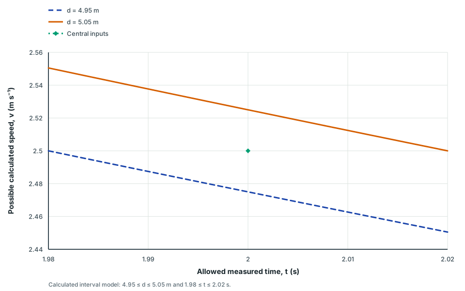
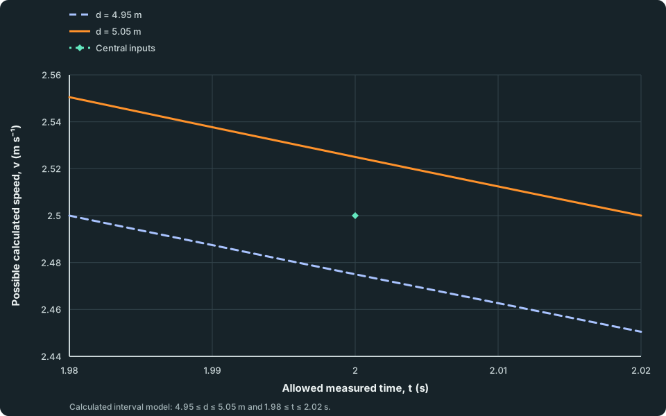
For time from 1.98 to 2.02 seconds, both possible-speed curves decrease. Distance 4.95 metres gives the lower curve and 5.05 metres the upper. The central inputs give 2.50 metres per second. The overall extremes are about 2.4505 and 2.5505 metres per second.
Scroll across the figure to read all labels.
View figure data
| Series | Allowed measured time, t (s) | Possible calculated speed, v (m s⁻¹) |
|---|---|---|
| d = 4.95 m | 1.980 | 2.500 |
| d = 4.95 m | 1.984 | 2.495 |
| d = 4.95 m | 1.988 | 2.490 |
| d = 4.95 m | 1.992 | 2.485 |
| d = 4.95 m | 1.996 | 2.480 |
| d = 4.95 m | 2.000 | 2.475 |
| d = 4.95 m | 2.004 | 2.470 |
| d = 4.95 m | 2.008 | 2.465 |
| d = 4.95 m | 2.012 | 2.460 |
| d = 4.95 m | 2.016 | 2.455 |
| d = 4.95 m | 2.020 | 2.450 |
| d = 5.05 m | 1.980 | 2.551 |
| d = 5.05 m | 1.984 | 2.545 |
| d = 5.05 m | 1.988 | 2.540 |
| d = 5.05 m | 1.992 | 2.535 |
| d = 5.05 m | 1.996 | 2.530 |
| d = 5.05 m | 2.000 | 2.525 |
| d = 5.05 m | 2.004 | 2.520 |
| d = 5.05 m | 2.008 | 2.515 |
| d = 5.05 m | 2.012 | 2.510 |
| d = 5.05 m | 2.016 | 2.505 |
| d = 5.05 m | 2.020 | 2.500 |
| Central inputs | 2.000 | 2.500 |
The graph shows every speed the inputs allow. At a fixed distance, a larger time gives a smaller speed, so the highest speed is at the top left and the lowest at the bottom right. Working out the limits like this is called numerical substitution. It is the safest method when the uncertainties are large or the formula is awkward, because the rules above are only approximations for small uncertainties.
Guided practice 2
A difference times a force
Problem
The moment M = (a-b)F is calculated from a = (0.120±0.001) m, b = (0.100±0.001) m and F = (3.00±0.03) N. Find the central difference and its absolute uncertainty, the fractional uncertainty in M, then M and its absolute uncertainty. Enter the absolute uncertainty before rounding the reported result.
Work through one operation at a time
Show the steps Optional working
Show the steps Optional working
Hints
Hint 1
the difference first
Which operation must you complete before multiplying by F?
Hint 2
then the product
M is a product of (a-b) and F, so add their fractional uncertainties.
Show solution step by step
The difference
Reason
Absolute uncertainties add for a difference.Working
Answer
a-b = (0.020±0.002) m, a fractional uncertainty of 0.10.
The product
Working
Answer
M = (0.020)(3.00) = 0.060 N m and (Δ M)/M = 0.10 + 0.03/3.00 = 0.11, so Δ M = 0.11 × 0.060 = 0.0066 N m. The result is (0.060±0.007) N m.
Check your understanding 1
The area of a circle is found from its radius, r = (2.00±0.05) cm, using A = π r². Find the area with its percentage and absolute uncertainties. Enter the absolute uncertainty to two significant figures before rounding the final reported result.
Show the steps Optional working
Show answer
A = π(2.00)² = 12.6 cm². The radius has a 2.5% uncertainty, and squaring doubles it, so the area has a 5.0% uncertainty: Δ A = 0.050 × 12.57 = 0.63 cm². The area is (12.6±0.6) cm². π is exact, so it adds no uncertainty.
Spot the mistake 3
A square root halves the percentage uncertainty
Learner claim
A speed is calculated from v = square root of 2gh, with h = (2.00±0.01) m and g taken as exact. A learner says v has the same 0.5% uncertainty as h. Find the percentage uncertainty in v before rounding.
Calculate the percentage uncertainty
Show solution step by step
Find the percentage uncertainty in h
Reason
The power rule works with fractional or percentage uncertainties.Working
Answer
0.01/2.00 × 100% = 0.5%
Apply the power
Working
Answer
v ∝ h^(1/2), so the percentage uncertainty in v is 1/2 × 0.5% = 0.25%.
Common mistake
Copying the input percentage ignores the power. A square root changes more slowly than its input, so its percentage uncertainty is smaller.
Check your understanding 2
A quantity x = 2.0±1.0 is used to calculate y = 1/x. Find the largest and smallest values of y. Compare the asymmetry with the public answer and explain why the fractional rule is unreliable in the next activity.
Show answer
x lies between 1.0 and 3.0, so y lies between 1/3.0 = 0.33 and 1/1.0 = 1.0, with a best value of 0.50. The range is lopsided: + 0.50 but only -0.17. The rule assumes a small uncertainty, but 50% is not small, so it cannot describe this range. Numerical substitution can.
Check your understanding 3
Why does the small-uncertainty rule fail to describe y = 1/x for x = 2.0±1.0? Use the central value and limits in your explanation.
Show answer
The best value is 0.50, with limits 0.33 and 1.0: the deviations are about −0.17 and +0.50. The input uncertainty is 50%, so a linear small-change approximation is poor. Numerical substitution exposes the asymmetric range rather than imposing a symmetric allowance.
Check your understanding 4
A learner calculates q = x-x, where both terms are the same measurement x, and gives Δ q = 2Δ x. What is wrong?
Show answer
x-x is exactly zero whatever the value of x, so q has no uncertainty. The rule assumes the two quantities can be wrong in different directions, but one measurement cannot be too large and too small at once. The rules apply to separately measured quantities.
Check your understanding 5
The lab calculates cylinder density from ρ = 4m/(π d²h). Use one reading, a metre rule for the diameter and vernier callipers for the length. Before opening the model, predict how changing only the diameter tool to a micrometer changes the diameter’s contribution to percentage uncertainty.
Show answer
The diameter allowance drops from ±1 mm to ±0.01 mm, so its fractional contribution falls. The power remains two, and division still adds a positive worst-case percentage allowance.
Test the input contributions
Select Cylinder density, set Repeat readings to 1, choose the metre rule for diameter and vernier callipers for length. Record the input contributions, then change only the diameter tool to the micrometer. The lab uses the larger of its stated instrument allowance and half the reading range; it does not calculate statistical uncertainty in a mean.
ρ = 4m / (πd²h), so %ρ ≈ %m + 2%d + %h. d readings: 12.7 mm; h readings: 30 mm; m readings: 31.9 g. Here % denotes percentage uncertainty. Each input uses the larger of its stated instrument allowance and half the reading range, not statistical uncertainty in a mean. Uniform-cylinder model with separately varying input allowances; product and power estimates are first-order. The approximate result is ρ = 8.4 ± 0.4 g cm⁻³.
- Result
- ρ = 8.4 ± 0.4 g cm⁻³
- Estimated percentage uncertainty
- 5.2 %
- Input contributions
- m: 0.31%; d²: 1.6%; h: 3.3%
- Rounded input estimates
- d: 12.7 ± 0.1 mm; h: 30 ± 1 mm; m: 31.9 ± 0.1 g
- Input allowance model
- Larger of stated instrument allowance and half the reading range
- Model assumptions
- Uniform cylinder; separately varying allowances; first-order estimate
Try this
0 of 4 doneMeasure the diameter with a metre rule, then with a micrometer. Watch the d² bar. (not done yet)
Squaring d doubles its fractional contribution. Compare every input contribution before choosing which measurement to improve.
Get the percentage uncertainty in the density below 1%. (not done yet)
Improve the biggest contribution first; making a small one smaller hardly helps.
Take five or more repeat readings of the diameter with the micrometer. (not done yet)
More readings can reveal a larger spread. This model uses the larger of the stated instrument allowance and half-range; it does not calculate statistical uncertainty in a mean.
Make the spring's extension large enough that its uncertainty is under 5%. (not done yet)
For separately varying input allowances, absolute uncertainties add in a difference. A larger extension reduces their percentage contribution; a shared additive offset would cancel.
You’ve tried every task.
Check your understanding 6
Record the two sets of contributions. Did the largest contribution change? Explain why a better diameter instrument eventually gives little benefit unless another measurement improves. You may keep your table on paper.
Show answer
Initially, diameter contributes about 15%, far above mass and length (each about 0.3%). With the micrometer, diameter contributes about 0.16%, while length and mass remain about 0.3% each. The total falls from about 16% to about 0.8%; length becomes the largest contribution. Further improvements to diameter leave the mass and length allowances, so those inputs now limit improvement. Compare your table, changed contribution, largest contribution and explanation.
Exam-style question 1
The acceleration of free fall from a pendulum
Examination question
A pendulum of length l = (0.800±0.002) m takes (36.0±0.2) s for 20 oscillations. The acceleration of free fall is found from g = 4π²l/T².
(a) Calculate g. [1 mark]
(b) Find the absolute uncertainty in g, and state g with its uncertainty. [3 marks]
Write your working before viewing the mark scheme
Show the steps Optional working
Show the steps Optional working
Show the steps Optional working
Show solution step by step
Calculate g
1 markMethod
Find the period, then substitute.Reason
The period is the time for one oscillation.Working
Answer
T = 36.0/20 = 1.80 s, so g = 4π²(0.800)/(1.80)² = 9.75 m s⁻².
Combine the fractional uncertainties
2 marksMethod
Add the fractional uncertainty in l to twice that in T.Reason
g is proportional to l and to T⁻²; 4π² is exact.Working
Answer
(Δ T)/T = 0.2/36.0 = 0.0056, the same as for the total time. So (Δ g)/g = 0.002/0.800 + 2(0.2/36.0) = 0.0025 + 0.0111 = 0.0136.
State the result
1 markWorking
Answer
Δ g = 0.0136 × 9.75 = 0.13 m s⁻², so g = (9.75±0.13) m s⁻². Keep two significant figures in the uncertainty because its first digit is 1; match the value to its decimal place.
Self-mark with the mark scheme
Tick each mark point that your answer includes.
Self-mark one point for each statement.
Check your understanding 7
Show the complete pendulum calculation on paper or below. Explain why timing 20 oscillations changes the absolute period uncertainty but not its fractional uncertainty, and report g with matching decimal places.
Show answer
T = 36.0/20 = 1.80 s and Δ T = 0.2/20 = 0.01 s, so Δ T/T = 0.2/36.0. The count is exact. g = 4π²(0.800)/(1.80)² = 9.75 m s⁻². Add 0.002/0.800 + 2(0.2/36.0) = 0.0136; multiplying by the unrounded g gives 0.13 m s⁻². Report (9.75±0.13) m s⁻². Compare the period, power factor, fraction-to-absolute step and final decimal places.
Timing 20 oscillations instead of one keeps the same 0.2 s timing uncertainty but spreads it over a time twenty times longer, so the fractional uncertainty in T is twenty times smaller.
Common mistakes
- Subtracting uncertainties when quantities are subtracted. For separately varying inputs, absolute uncertainties add.
- Adding absolute uncertainties for a product or quotient. Use fractional uncertainties.
- Forgetting to multiply by the power: T² doubles the fractional uncertainty in T.
- Giving an uncertainty to an exact number such as π or 1/2.
- For the largest value of a quotient, using the largest denominator instead of the smallest.
Before you move on
Check your understanding 8
Two separately measured lengths are a = (4.00±0.10) m and b = (2.00±0.20) m. Find the uncertainty in a-b and estimate the percentage uncertainty in a/b. Then find the largest possible value of a/b by substitution.
Show the steps Optional working
Show answer
For the difference, add absolute uncertainties: a-b = (2.00±0.30) m. For the quotient, add fractional uncertainties: 0.10/4.00 + 0.20/2.00 = 0.125, or 12.5%. Its largest possible value is 4.10/1.80 = 2.28, using the largest numerator and smallest denominator.
Spotted an error? Report a correction
Syllabus and review details
- GCE A-Level H2 Physics 2027 · 2027
Content Overview, PDF pages 9–10; Subject Content, PDF pages 11–30
Last reviewed: