Wavefunctions of a Particle Trapped Within a Box

In an infinite square well, the wavefunction must vanish at the walls. This forces standing-wave solutions and leads to discrete ψₙ(x).

1. Schrödinger equation inside the box

Inside the box ( 0 < x < L), V(x) = 0, so the time-independent Schrödinger equation becomes:

-(ħ²/2m)d²ψ/dx² = Eψ

Define k² = 2mE/ħ², giving:

d²ψ/dx² = -k²ψ

The general solution is:

ψ(x) = A sin(kx) + B cos(kx)

2. Apply the boundary conditions

For an infinite wall, the wavefunction must vanish at the boundary:

• ψ(0) = 0, so B = 0.
• ψ(L) = 0, so sin(kL) = 0 and therefore kL = nπ.

So

k = nπ/L (n = 1,2,3,…)

and the stationary-state wavefunctions inside the well are:

ψₙ(x) = A sin((nπ x)/L) (0 < x < L)

Outside the well:

ψₙ(x) = 0 (x ≤ 0 or x ≥ L)

3. Normalisation constant

The constant A is fixed by ∫₀^L |ψₙ(x)|² dx = 1:

A = square root of (2/L)

So the standard result is:

ψₙ(x) = square root of (2/L) sin((nπ x)/L) (0 < x < L)

4. Probability density and nodes

The probability density is:

|ψₙ(x)|² = 2/L sin² ((nπ x)/L)

Nodes occur where ψₙ = 0:

• always at x = 0 and x = L
• plus n-1 interior nodes at x = mL/n for m = 1,2,…,n-1

Probability density |ψn|² in a 1D box (shape only)

Example shapes of |ψn(x)|² for n = 1 and n = 2 in a 1D infinite square well (0 ≤ x/L ≤ 1).

Scroll across the graph to read all labels.

Open full-size graph

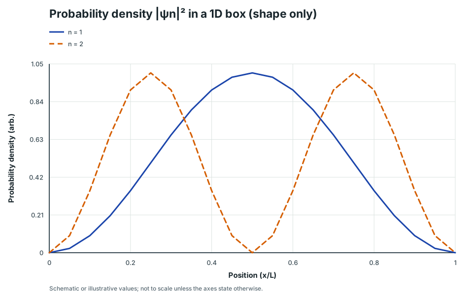
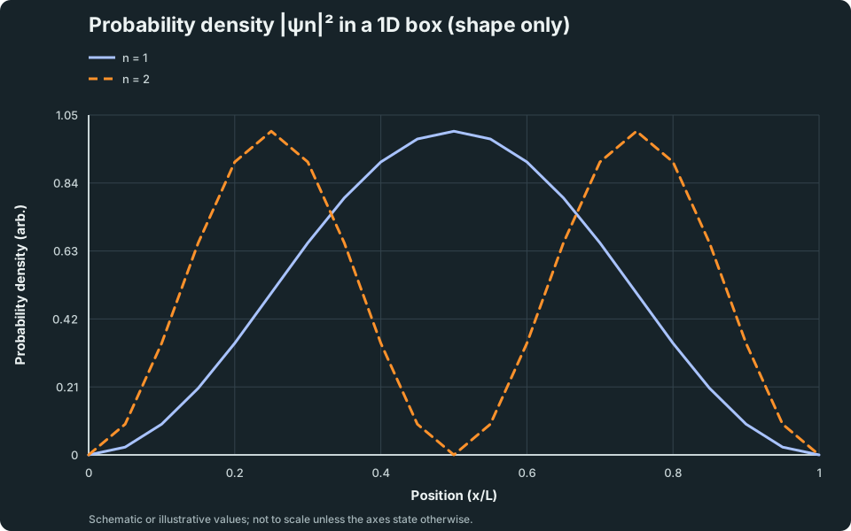
View figure data

Values for Probability density |ψn|² in a 1D box (shape only)

Position (x/L)	n = 1	n = 2
0	0	0
0.05	0.024	0.095
0.1	0.095	0.345
0.15	0.206	0.655
0.2	0.345	0.905
0.25	0.5	1
0.3	0.655	0.905
0.35	0.794	0.655
0.4	0.905	0.345
0.45	0.976	0.095
0.5	1	0
0.55	0.976	0.095
0.6	0.905	0.345
0.65	0.794	0.655
0.7	0.655	0.905
0.75	0.5	1
0.8	0.345	0.905
0.85	0.206	0.655
0.9	0.095	0.345
0.95	0.024	0.095
1	0	0

Values for Probability density |ψn|² in a 1D box (shape only)

Position (x/L)	n = 1	n = 2
0	0	0
0.05	0.024	0.095
0.1	0.095	0.345
0.15	0.206	0.655
0.2	0.345	0.905
0.25	0.5	1
0.3	0.655	0.905
0.35	0.794	0.655
0.4	0.905	0.345
0.45	0.976	0.095
0.5	1	0
0.55	0.976	0.095
0.6	0.905	0.345
0.65	0.794	0.655
0.7	0.655	0.905
0.75	0.5	1
0.8	0.345	0.905
0.85	0.206	0.655
0.9	0.095	0.345
0.95	0.024	0.095
1	0	0

5. Common traps

1. Writing ψₙ(x) = A sin(nπ/L)x (the x must be inside the sine).
2. Using h instead of ħ in the Schrödinger equation.
3. Forgetting ψ = 0 at the walls for an infinite well.
4. Confusing ψ with |ψ|² (probability density).

6. Worked Examples

7. Quick check