Particle Trapped in a Box of Length L

This is the classic infinite square well model: a particle (e.g., an electron) is trapped in a 1D region of length L. It is the cleanest example of how boundary conditions lead to discrete standing wavelengths, energies, and possible momentum magnitudes.

1. Model and assumptions

We idealise the walls as infinitely high:

• Inside the box ( 0 < x < L): V(x) = 0 (a constant).
• Outside the box: V(x) → ∞ (so the particle cannot exist there).

The potential sketch below is the setup used throughout particle-in-a-box derivations: zero potential inside, effectively infinite walls outside.

2. Infinite-wall boundary conditions

Because V → ∞ outside the box, the probability of finding the particle outside must be zero:

• ψ(x) = 0 for x ≤ 0 and x ≥ L.
• The wavefunction must also vanish at the walls: ψ(0) = ψ(L) = 0.

This “node at each wall” condition is the key reason energy becomes discrete.

3. Standing-wave quantisation

Inside the well, the particle behaves like a standing wave with nodes at both ends. Therefore, the box length must fit an integer number of half-wavelengths:

L = nλₙ/2 (n = 1,2,3,…)

where λₙ is the de Broglie wavelength for the nth state.

Using λ = h/|p| identifies the magnitude associated with each pair of travelling-wave components:

|pₙ| = nh/2L

The standing energy eigenstate is not a state of one definite momentum. A momentum measurement gives + pₙ or -pₙ with equal probability, while either result gives the same pₙ² and therefore the same energy:

Eₙ = pₙ²/2m = n²h²/8mL² = n²π²ħ²/2mL²

Derivations and full forms:

• Allowed Energy States of a Trapped Particle
• Wavefunctions of a Particle Trapped Within a Box

Standing-wave modes in a 1D box (shape of ψn)

Example shapes of the wavefunction ψn(x) for n = 1 and n = 2 in a 1D infinite square well (0 ≤ x/L ≤ 1), showing nodes at the walls and additional nodes for higher n.

Scroll across the graph to read all labels.

Open full-size graph

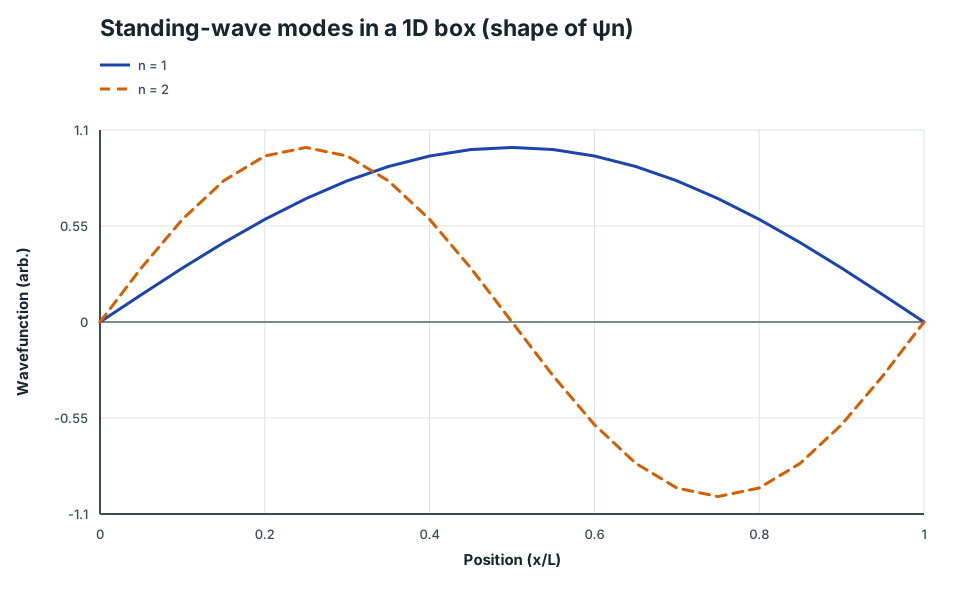
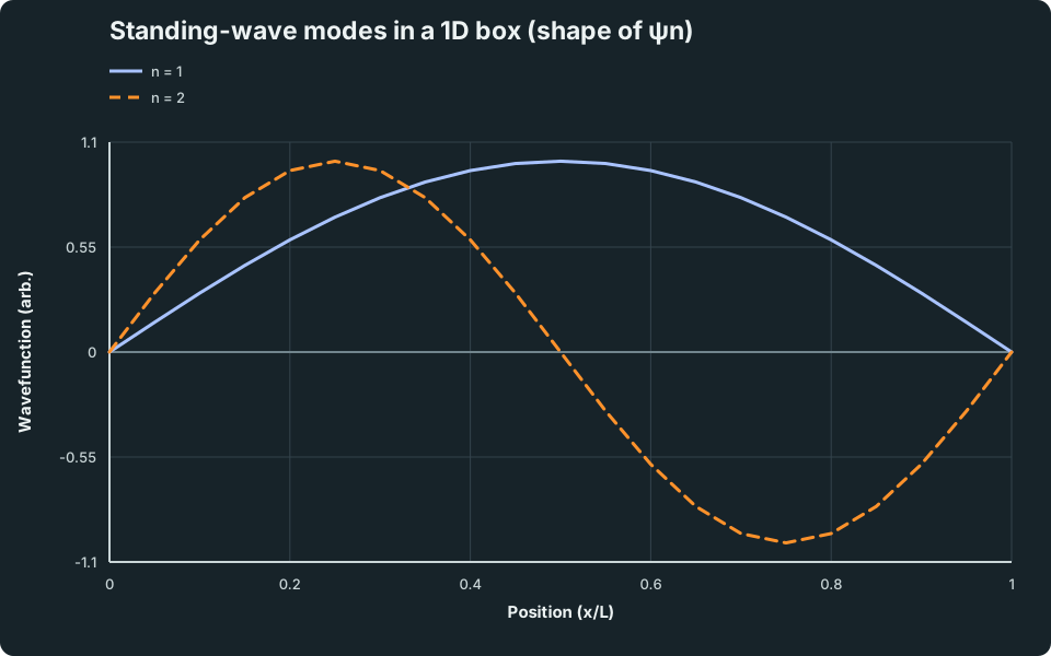
View figure data

Values for Standing-wave modes in a 1D box (shape of ψn)

Position (x/L)	n = 1	n = 2
0	0	0
0.05	0.156	0.309
0.1	0.309	0.588
0.15	0.454	0.809
0.2	0.588	0.951
0.25	0.707	1
0.3	0.809	0.951
0.35	0.891	0.809
0.4	0.951	0.588
0.45	0.988	0.309
0.5	1	0
0.55	0.988	-0.309
0.6	0.951	-0.588
0.65	0.891	-0.809
0.7	0.809	-0.951
0.75	0.707	-1
0.8	0.588	-0.951
0.85	0.454	-0.809
0.9	0.309	-0.588
0.95	0.156	-0.309
1	0	0

Values for Standing-wave modes in a 1D box (shape of ψn)

Position (x/L)	n = 1	n = 2
0	0	0
0.05	0.156	0.309
0.1	0.309	0.588
0.15	0.454	0.809
0.2	0.588	0.951
0.25	0.707	1
0.3	0.809	0.951
0.35	0.891	0.809
0.4	0.951	0.588
0.45	0.988	0.309
0.5	1	0
0.55	0.988	-0.309
0.6	0.951	-0.588
0.65	0.891	-0.809
0.7	0.809	-0.951
0.75	0.707	-1
0.8	0.588	-0.951
0.85	0.454	-0.809
0.9	0.309	-0.588
0.95	0.156	-0.309
1	0	0

4. Interpretation

• Quantisation comes from boundary conditions. The walls force nodes, which force discrete λₙ, hence discrete pₙ and Eₙ.
• The energy is definite in a stationary state, but the momentum direction is not: the two outcomes are + pₙ and -pₙ.
• n = 0 is not allowed (it would imply λ → ∞ and ψ = 0 everywhere).
• Higher n gives higher energy and more nodes (more oscillations).

5. Common traps

1. Writing n = 0 as the ground state (ground state is n = 1).
2. Mixing up “half-wavelengths in the box” ( L = nλ/2) with “full wavelengths” ( L = nλ).
3. Confusing ψ with |ψ|² (probability density).
4. Forgetting to state boundary conditions explicitly when asked “why quantised?”.
5. Treating pₙ as one signed momentum rather than the magnitude of the two possible outcomes.

6. Quick check

A. Without calculating anything, what is E₂/E₁ for a particle in a 1D box?

B. Why is n = 0 not allowed?